This is the code companion to
formalization/NonlinearDynamics/Random/ComplexGaussian.lean. Every named
declaration in that file is explained below. The compiler-checked source is
the authority whenever prose notation abbreviates a Lean type.
The reusable probability background lives in Gaussian Laws, Independence, and Normalization. The geometric continuation is Complex Gaussian Coordinates and Geometry. Useful compact entries include Gaussian distribution , variance , independence , normalization convention , and Cartesian complex Gaussian law .
Choose a route up
| Route | Begin with | Destination |
|---|---|---|
| First complex-probability encounter | Base camp | See a complex variable as a two-dimensional real random vector |
| Measure-theory route | Build the law | Follow product measure, measurable map, and exact marginals |
| Lean route | Declaration map | Match every theorem to its upstream proof engine |
| Geometry route | What Cartesian structure entails | Separate an axis-aligned ellipse from circular or proper symmetry |
| Physics route | Quadratures and matrix entries | Connect coordinate variances to complex amplitudes and future GUE entries |
| Edge-case route | Degenerate laws | Understand line-supported and point-supported Gaussians |
Learning objectives
By the summit, a reader should be able to:
- construct a complex law by mapping a product law through the real-linear equivalence \(\mathbb R^2\simeq\mathbb C\);
- explain why
cartesianComplexGaussian m vRe vImexposes two variances; - distinguish the law of a complex variable from a sample map into \(\mathbb C\);
- recover exact real and imaginary marginal laws by mapping back through coordinate projections;
- explain why marginal laws alone do not prove independence;
- interpret
HasGaussianLaw Z Pover \(\mathbb C\) as real-vector-space Gaussianity; - derive finite moments, integrability, and expectation from the exact law;
- explain the line-supported and double-degenerate cases without dividing by a variance;
- state exactly what
of_indep_re_imassumes about two source variables; - distinguish Cartesian, circular, proper, and isotropic language;
- compute the normalization ledger for the two common equal-variance choices;
- identify every theorem still required before an object may be called GUE.
The construction in one picture
flowchart LR
  A["real Gaussian for the real coordinate"] --> C["product law on an ordered pair"]
  B["real Gaussian for the imaginary coordinate"] --> C
  C --> D["continuous real-linear equivalence"]
  D --> E["exact Cartesian law on the complex plane"]
  E --> F["recover exact real marginal"]
  E --> G["recover exact imaginary marginal"]
  E --> H["recover coordinate independence"]
  E --> I["real-vector-space Gaussianity and finite moments"]
  J["equal coordinate variances"] -. "future symmetry theorem" .-> K["circular centered law"]
  L["matrix variance ledger"] -. "future ensemble theorem" .-> M["GUE law"]
Reading the proof graph. The solid arrows are the current checked interface: product real laws are transported to the complex plane, and the exact coordinate facts can be recovered. The dotted arrows are deliberately absent. Equal variances suggest additional rotational geometry, while a matrix ledger can eventually support GUE, but neither claim is made by this module.
Why a complex Gaussian needs two coordinates
A real Gaussian variable lives on a line. A complex Gaussian variable lives on a plane. Writing
\[ Z=X+iY \]identifies that plane with two real coordinate axes. The formula is elementary, but its probabilistic content is not. One must still say:
- the law of \(X\);
- the law of \(Y\);
- whether \(X\) and \(Y\) are independent;
- whether their variances are equal;
- which convention turns those coordinate variances into a complex scale; and
- what happens when one or both variances are zero.
The phrase “complex Gaussian” is used with several conventions across probability, statistics, signal processing, and random-matrix physics. The classical multivariate setting already makes the complex structure explicit (Goodman 1963). A formal interface should therefore preserve the raw facts before introducing a convenience name. This module chooses the descriptive adjective Cartesian: the law is built in a named pair of axes from independent real Gaussian coordinates.
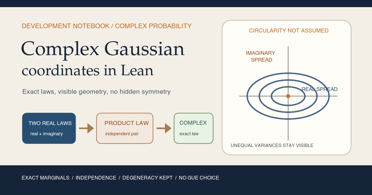
That choice is intentionally broader than the most familiar circular complex normal. If the coordinate variances differ, contours are ellipses rather than circles. If one variance vanishes, the law is supported on a line. If both vanish, it is supported at a single point. All three situations are legitimate values of the same parameterized measure.
Lineage, local contribution, and nonclaims
Product measures, Gaussian measures on real normed spaces, measurable linear images, and independence are established mathematics. The repository pins Mathlib 4.32.0 at a specific commit (Mathlib release), which supplies the foundational theorems. The project module does not reprove the Gaussian integral, derive a bivariate density, or develop characteristic functions from scratch.
The local contribution is a random-matrix-facing interface:
- an exact complex measure with named mean and separate coordinate variances;
- an exact-law predicate around that measure;
- forward construction from the product of real laws;
- backward recovery of the pair law and both marginals;
- a theorem recording independence of real and imaginary parts;
- qualitative Gaussianity over the real vector space \(\mathbb C\);
- finite-moment, integrability, and complex-mean consequences;
- explicit double-degenerate Dirac and almost-everywhere-constant behavior;
- and a constructor from arbitrary independent real variables with exact laws.
Not claimed
Cartesiandoes not mean circular symmetry under multiplication by every complex phase.Cartesiandoes not mean properness or vanishing pseudo-covariance.- Unequal coordinate variances are not rejected or normalized away.
- No density formula on \(\mathbb C\) is introduced.
- No complex variance notation is selected.
- No covariance matrix or pseudo-covariance API is introduced.
- No ordinary measurability of the source variables is inferred from
HasLaw. - No matrix, Hermitian ensemble, Wigner matrix, or GUE law is constructed.
- No diagonal or off-diagonal dimension scaling is selected.
- No unitary invariance, eigenvalue law, trace expectation, or asymptotic result follows from this file.
Base camp: one complex number, two real coordinates
Every \(z\in\mathbb C\) has unique coordinates
\[ z=\operatorname{Re}(z)+i\operatorname{Im}(z). \]The library represents this decomposition as a continuous real-linear equivalence:
Complex.equivRealProdCLM : ℂ ≃L[ℝ] ℝ × ℝ
Its forward direction sends \(z\) to (z.re, z.im). Its inverse sends a pair
p to p.1 + p.2 * Complex.I. The CLM suffix signals continuous linear
structure. That one object provides several facts the probability proof needs:
- it is a bijection;
- both directions are real-linear;
- both directions are continuous;
- therefore both directions are Borel measurable; and
- qualitative Gaussianity is preserved under this equivalence.
This equivalence and its inverse formula are part of Mathlib’s checked complex analysis API (Mathlib complex source). This is more than a convenient conversion function. It says that complex Gaussianity in this file is Gaussianity on the two-dimensional real normed space underlying \(\mathbb C\). The definition does not assume complex linearity.
Camp one: build the law before naming the variable
Fix a complex mean \(m\) and two nonnegative real variances \(v_{\mathrm{Re}}\) and \(v_{\mathrm{Im}}\). The coordinate measures are Mathlib’s exact variance-parameterized real Gaussians (Mathlib real Gaussians). First build the product measure
\[ \gamma =\mathcal N\!\left(\operatorname{Re}m,v_{\mathrm{Re}}\right) \otimes \mathcal N\!\left(\operatorname{Im}m,v_{\mathrm{Im}}\right) \]on \(\mathbb R\times\mathbb R\). Mathlib’s Measure.prod supplies the exact
measure construction and marginal theorems
(Mathlib product measures). Then push it through
\(T(x,y)=x+iy\):
Here \(T_{\#}\gamma\) means the pushforward measure. For every measurable set \(A\subseteq\mathbb C\), it assigns the mass \(\gamma(T^{-1}(A))\).
cartesianComplexGaussian
cartesianComplexGaussian m vRe vIm is exactly that mapped product measure.
Its three parameters remain visible. In particular, no function combines
vRe and vIm into a single ambiguous number called variance.
The definition uses Measure.map only after supplying a measurable inverse
coordinate equivalence. This matters because Mathlib’s Measure.map is total:
outside the measurable case it has fallback behavior. The proof never relies
on that fallback.
instIsProbabilityMeasureCartesianComplexGaussian
The named probability instance
instIsProbabilityMeasureCartesianComplexGaussian closes the probability
bookkeeping loop. Each real Gaussian is a probability measure. Their product
is a probability measure. Mapping a probability measure through a measurable
function preserves total mass one. Later expectation and HasGaussianLaw
theorems can therefore obtain the required typeclass automatically.
This theorem does not say the measure is absolutely continuous. When either coordinate variance is zero, the measure is singular with respect to two-dimensional Lebesgue measure, yet it remains a probability measure.
cartesianComplexGaussian_map_equivRealProd
cartesianComplexGaussian_map_equivRealProd proves that transporting the
complex law through
Complex.equivRealProdCLM recovers the original product of real Gaussian
measures. Conceptually,
The proof uses measurability in both directions and the inverse laws of the equivalence. This is the central audit theorem for the definition: the mapped measure has not forgotten or mixed the two coordinates.
cartesianComplexGaussian_map_re and cartesianComplexGaussian_map_im
The two coordinate map declarations cartesianComplexGaussian_map_re and
cartesianComplexGaussian_map_im prove
and
\[ (\operatorname{Im})_{\#} \operatorname{CG}_{\mathrm{cart}}(m,v_{\mathrm{Re}},v_{\mathrm{Im}}) =\mathcal N(\operatorname{Im}m,v_{\mathrm{Im}}). \]The map-back theorem exposes the product law; Measure.map_fst_prod and
Measure.map_snd_prod then recover its marginals. These are exact statements,
not merely assertions that the coordinates are qualitatively Gaussian.
instIsGaussianCartesianComplexGaussian
instIsGaussianCartesianComplexGaussian records that the exact Cartesian
measure is also Gaussian as a measure on the real normed
space \(\mathbb C\). Mathlib defines this measure class through every real
continuous linear projection
(Mathlib Gaussian measures). The proof starts
with the product of two Gaussian real
measures and transports Gaussianity through the continuous real-linear
equivalence.
This theorem is geometric but parameter-forgetting. It enables generic Gaussian tools, while the exact mapped-product definition retains the means, coordinate variances, and independence needed for matrix construction.
Camp two: exact law of a complex sample map
A measure on \(\mathbb C\) is not yet a random variable. Let \((\Omega,\mathcal F,P)\) be a measure space and \(Z:\Omega\to\mathbb C\) a sample map.
HasCartesianComplexGaussianLaw
HasCartesianComplexGaussianLaw Z m vRe vIm P abbreviates the exact statement
HasLaw Z (cartesianComplexGaussian m vRe vIm) P
The predicate records two things inherited from HasLaw
(Mathlib law API):
Zis almost-everywhere measurable underP;- pushing
Pforward throughZgives exactly the requested Cartesian law.
The second item is stronger than separately naming the two marginal laws. It fixes the joint distribution, including independence.
HasCartesianComplexGaussianLaw.aemeasurable
The aemeasurable declaration exposes the first HasLaw field. It returns
AEMeasurable Z P, not Measurable Z.
Almost-everywhere measurability is the right law-level notion because changing
Z on a P-null set should not change its probability law. Ordinary
measurability is a stronger pointwise statement and is not fabricated by this
wrapper.
HasCartesianComplexGaussianLaw.isProbabilityMeasure
The source-normalization declaration proves that an exact Cartesian complex
Gaussian law forces P to be a probability measure. The target law has mass
one, and equality of pushforward laws transports that mass back to the source.
As in the real primitive, this is a consequence of the exact law, not a global assumption baked into the predicate’s definition.
Camp three: recover the coordinates and their dependence
The exact complex law contains a complete statement about the ordered pair
(Z.re, Z.im). The next declarations unpack it at progressively smaller
scales.
HasCartesianComplexGaussianLaw.jointHasLaw
HasCartesianComplexGaussianLaw.jointHasLaw states that
fun omega => ((Z omega).re, (Z omega).im)
has the product law
(gaussianReal m.re vRe).prod (gaussianReal m.im vIm)
under P. It composes the exact law of Z with the forward
Complex.equivRealProdCLM map, then simplifies using the map-back theorem.
This theorem is the strongest coordinate-level statement in the file. The marginal and independence declarations can be read as projections of it.
HasCartesianComplexGaussianLaw.real_hasLaw
HasCartesianComplexGaussianLaw.real_hasLaw yields
HasRealGaussianLaw (fun omega => (Z omega).re) m.re vRe P
It may be proved by composing the joint pair law with Prod.fst, or by
composing Z directly with Complex.re and applying the measure-level map
theorem. Either path preserves a.e. measurability and identifies the exact
pushforward law.
HasCartesianComplexGaussianLaw.imag_hasLaw
HasCartesianComplexGaussianLaw.imag_hasLaw is the parallel theorem for
Complex.im:
HasRealGaussianLaw (fun omega => (Z omega).im) m.im vIm P
The separate theorem is not redundant. Random-matrix code will later assign different variance schedules to real and imaginary coordinates, and it should be able to retrieve each schedule directly.
HasCartesianComplexGaussianLaw.indep_re_im
HasCartesianComplexGaussianLaw.indep_re_im proves
IndepFun (fun omega => (Z omega).re)
  (fun omega => (Z omega).im) P
The proof uses the exact product joint law and Mathlib’s law-level characterization of independent functions (Mathlib independence API). This is the right logical direction: a product joint law entails independence. Merely knowing that each marginal is Gaussian would not.
For example, if \(X\) is a real Gaussian and \(Y=X\), then both coordinates have Gaussian marginals but are maximally dependent. The product-law theorem rules that example out.
Camp four: Gaussian consequences in the complex plane
HasCartesianComplexGaussianLaw.hasGaussianLaw
The qualitative declaration drops the explicit parameters and proves
HasGaussianLaw Z P
for the real normed vector space \(\mathbb C\). Any real continuous linear
functional applied to Z therefore has a real Gaussian law.
The exact predicate should remain the default while normalization information matters. The qualitative theorem is the bridge to Mathlib’s general Gaussian integrability and linear-image API.
HasCartesianComplexGaussianLaw.memLp
For every extended exponent p with p ≠ ⊤, the memLp declaration proves
MemLp Z p P
This includes every finite positive moment exponent and Mathlib’s special
p = 0 case. It excludes p = ∞, because a nondegenerate Gaussian variable
is not essentially bounded.
The proof does not integrate a two-dimensional density in this project. It
passes through hasGaussianLaw and reuses Mathlib’s general Gaussian moment
theorem (Mathlib Gaussian variables).
HasCartesianComplexGaussianLaw.integrable
Integrability is the \(L^1\) specialization needed to define the Bochner expectation
\[ \int_\Omega Z(\omega)\,dP(\omega). \]The theorem follows from the finite-moment result, but it deserves a named
declaration because later matrix-entry and trace arguments will require
Integrable directly.
HasCartesianComplexGaussianLaw.mean_eq
HasCartesianComplexGaussianLaw.mean_eq proves
This is a vector-valued integral in \(\mathbb C\). The proof can be audited
coordinatewise: the exact real-part law gives mean m.re, the exact
imaginary-part law gives mean m.im, and equality of complex numbers follows
from equality of both coordinates.
No single scalar called “complex variance” appears. The file has established
the expectation while continuing to store second-order scale as the ordered
pair (vRe, vIm).
Camp five: the degenerate cases are part of the space
cartesianComplexGaussian_zero_variances
At the measure level, cartesianComplexGaussian_zero_variances proves
Each real Gaussian becomes a Dirac measure at its coordinate mean. Their
product is the Dirac measure at (m.re, m.im), and the inverse coordinate map
sends that pair to m.
This is not a density theorem with a limiting argument. It is an exact identity at the boundary of the nonnegative variance parameters.
HasCartesianComplexGaussianLaw.ae_eq_const_of_variances_zero
HasCartesianComplexGaussianLaw.ae_eq_const_of_variances_zero proves that an
exact law with both
variances zero satisfies
It does not claim pointwise equality. A random variable may differ from m on
a null set while retaining the same Dirac law.
One zero variance
There is no special theorem that discards the cases (vRe, 0) or (0, vIm).
That omission is a feature. The general definition already handles them:
- if
vIm = 0, the law lies on the horizontal line with imaginary coordinatem.im; - if
vRe = 0, the law lies on the vertical line with real coordinatem.re; - if both are zero, the two lines meet at the Dirac point
m.
Retaining these cases keeps later coordinate schedules closed under zero scaling and allows sparse or boundary constructions without a second API.
Summit construction: start from independent real variables
HasCartesianComplexGaussianLaw.of_indep_re_im
Suppose two real sample maps satisfy exact laws
\[ X\sim\mathcal N(\operatorname{Re}m,v_{\mathrm{Re}}), \qquad Y\sim\mathcal N(\operatorname{Im}m,v_{\mathrm{Im}}), \]and suppose IndepFun X Y P. The constructor proves that
has HasCartesianComplexGaussianLaw with those exact parameters.
The proof has two clean transports:
IndepFun.hasLaw_prodturns the exact marginal laws and independence into the exact product law of(X, Y);HasLaw.compmaps that pair law throughComplex.equivRealProdCLM.symm.
The constructor asks for no ordinary Measurable X or Measurable Y
hypothesis. This is an important difference from the earlier
IndependentRealGaussianFamily record, which stores ordinary coordinate
measurability for later pointwise family operations. Here the task is only to
prove a law. The two HasRealGaussianLaw hypotheses provide a.e.
measurability, and IndepFun provides the dependence structure. The proof
derives IsProbabilityMeasure P from hX before invoking the finite-measure
product-law API. Its last step uses HasLaw.congr to identify the composed
equivalence with the displayed function X + Y * Complex.I almost everywhere.
What Cartesian structure entails, and what it does not
Center the variable by writing
\[ Z-m=U+iV, \]where \(U\) and \(V\) are independent, centered real Gaussians with variances \(v_{\mathrm{Re}}\) and \(v_{\mathrm{Im}}\). Then
\[ \mathbb E\lvert Z-m\rvert^2 =v_{\mathrm{Re}}+v_{\mathrm{Im}}. \]This paper calculation helps compare conventions, but the current Lean file does not package the left-hand side as a named complex variance theorem.
Another diagnostic is the centered pseudo-covariance, also called relation in some complex second-order literature (Picinbono 1996):
\[ \mathbb E[(Z-m)^2] =v_{\mathrm{Re}}-v_{\mathrm{Im}}, \]because independence and centering remove the mixed term. When the coordinate variances are equal, this expression vanishes. When they differ, it records the preferred axes of the ellipse. The current module does not formalize this identity or define properness, so it is mathematical orientation rather than a checked project theorem.
The vocabulary ladder is:
| Term | What it should mean here | Established by this file? |
|---|---|---|
| Cartesian | Exact independent real and imaginary Gaussian coordinates in the chosen axes | Yes |
| Isotropic covariance | Equal coordinate variances after centering | The parameters can express it; no named symmetry theorem |
| Proper | Vanishing pseudo-covariance or relation, under the chosen definition | No |
| Circular centered law | Invariance in distribution under every complex phase rotation | No |
| Standard complex Gaussian | A convention-dependent special case | Intentionally unnamed |
For a scalar Gaussian, equal independent centered coordinate variances are the familiar route to circular symmetry. Still, that implication deserves its own definition and proof. A name should not perform the proof’s work.
Why anisotropic laws are retained
An anisotropic complex Gaussian has different spreads along the real and imaginary axes. Its constant-density contours, when both variances are positive, are axis-aligned ellipses. Retaining this family is useful for more than generality’s sake:
- it makes every normalization choice explicit;
- it supports models with unequal quadrature noise;
- it exposes accidental real-imaginary asymmetry in later matrix entries;
- it keeps degenerate line-supported limits inside the same type;
- and it lets future theorems state equal-variance hypotheses exactly where rotational symmetry is used.
If the constructor had accepted only one variance parameter, equal splitting would already have been chosen. The current three-parameter measure prevents that hidden decision.
Why physicists care about the variance split
In wave mechanics and signal processing, a complex amplitude carries two quadratures. In random-matrix physics, an off-diagonal Hermitian entry also has two real degrees of freedom, while its conjugate partner is fixed and a diagonal entry must be real. Dyson’s symmetry-class program supplies the historical matrix-ensemble motivation (Dyson 1962); it does not choose the scalar normalization used here.
Two common centered equal-coordinate choices illustrate the convention trap.
Let U and V be independent real Gaussians.
| Coordinate variances | Resulting second moment | Common informal shorthand |
|---|---|---|
| \(\operatorname{Var}(U)=\operatorname{Var}(V)=1/2\) | (\mathbb E | U+iV |
| \(\operatorname{Var}(U)=\operatorname{Var}(V)=1\) | (\mathbb E | U+iV |
Both are mathematically coherent. Calling both “standard complex Gaussian” without a ledger creates a factor-of-two error.
A future Wigner-scaled GUE may use dimension-dependent variances, often with a real diagonal variance and half-sized real and imaginary off-diagonal variances. This project has not approved that convention, density exponent, trace normalization, or zero-dimensional policy. The current module provides the coordinates needed to state the choice later; it does not make the choice.
The entire Lean file as a declaration map
| Declaration | Layer | Checked content |
|---|---|---|
cartesianComplexGaussian | Measure definition | Map a product of exact real Gaussian measures into \(\mathbb C\) |
instIsProbabilityMeasureCartesianComplexGaussian | Measure structure | The mapped product has total mass one |
instIsGaussianCartesianComplexGaussian | Measure structure | The law is Gaussian over the real vector space \(\mathbb C\) |
cartesianComplexGaussian_map_equivRealProd | Exact measure identity | Real-imaginary coordinates recover the original product law |
cartesianComplexGaussian_map_re | Exact marginal | Real projection has gaussianReal m.re vRe |
cartesianComplexGaussian_map_im | Exact marginal | Imaginary projection has gaussianReal m.im vIm |
cartesianComplexGaussian_zero_variances | Degenerate measure | Two zero variances give Measure.dirac m |
HasCartesianComplexGaussianLaw | Exact sample-map predicate | HasLaw for the Cartesian complex measure |
HasCartesianComplexGaussianLaw.aemeasurable | Measurability | Exposes AEMeasurable Z P |
HasCartesianComplexGaussianLaw.isProbabilityMeasure | Source normalization | Exact law forces P to have mass one |
HasCartesianComplexGaussianLaw.jointHasLaw | Exact joint law | Coordinate pair has the product law |
HasCartesianComplexGaussianLaw.real_hasLaw | Exact coordinate law | Z.re has the named real Gaussian law |
HasCartesianComplexGaussianLaw.imag_hasLaw | Exact coordinate law | Z.im has the named real Gaussian law |
HasCartesianComplexGaussianLaw.indep_re_im | Dependence | Z.re and Z.im are IndepFun |
HasCartesianComplexGaussianLaw.hasGaussianLaw | Qualitative class | Every real linear projection is Gaussian |
HasCartesianComplexGaussianLaw.memLp | Moments | MemLp Z p P for p ≠ ⊤ |
HasCartesianComplexGaussianLaw.integrable | Integrability | Complex Bochner integrability |
HasCartesianComplexGaussianLaw.mean_eq | First moment | Integral of Z equals m |
HasCartesianComplexGaussianLaw.ae_eq_const_of_variances_zero | Degenerate sample map | Z = m almost everywhere |
HasCartesianComplexGaussianLaw.of_indep_re_im | Constructor | Independent exact real laws assemble into the complex exact law |
The source names are discussed in the surrounding subsections, and the proof-to-prose gate checks this final inventory mechanically.
Proof architecture: a small number of transports
1. Product first
The two real Gaussian probability measures are combined with Measure.prod.
This supplies the independent joint law before any map into \(\mathbb C\)
occurs.
2. Map through an equivalence
Complex.equivRealProdCLM.symm is continuous and measurable. Measure.map
therefore transports the product law into the complex plane without a density
calculation.
3. Map back to audit the definition
Measure.map_map and the inverse law for the equivalence recover the original
product. The marginal theorems then use the first and second projections.
4. Move between product law and independence
At measure level, a product is independent by construction. At sample-map
level, an exact product joint law implies IndepFun. In the constructor,
IndepFun.hasLaw_prod runs the bridge in the other direction.
5. Forget parameters only when useful
The exact law is converted to HasGaussianLaw only to reuse generic Gaussian
theorems such as finite MemLp. The public exact predicate remains available
for coordinate arithmetic.
6. Prove vector identities by coordinates
The complex mean and the double-zero conclusion reduce to real and imaginary facts, then close by complex extensionality. This proof style exposes exactly which coordinate theorem supplies each equality.
Exact commands: compile, cover, and preview
From the repository root on macOS or Linux:
source "$HOME/.elan/env"
cd formalization
lake env lean -DwarningAsError=true NonlinearDynamics/Random/ComplexGaussian.lean
lake build
cd ..
The direct lean command checks this module with every warning promoted to an
error. lake build checks the complete import graph.
Starting from the repository root, build the complete formalization and check the public teaching content:
cd formalization
lake build

cd ..
make content-hygiene
make site-check
lake build checks the complete project import graph. The final two commands
inspect the public teaching content and render the site.
Regenerate the card from any working directory:
site/content/development-notebook/2026/07/\
complex-gaussians-from-independent-real-coordinates/generate-card.sh
The generator resolves its default output beside itself, strips time-dependent PNG metadata, and checks the dimensions. It can also receive an explicit output path as its first argument for byte-identity testing.
Edge-case register
| Situation | What the checked API does | Common wrong inference |
|---|---|---|
vRe = 0, vIm > 0 | Supports a vertical Gaussian line through m | Every complex Gaussian has a planar density |
vRe > 0, vIm = 0 | Supports a horizontal Gaussian line through m | Both coordinates must be nondegenerate |
vRe = vIm = 0 | Measure is dirac m; sample map equals m a.e. | The definition is undefined at zero variance |
vRe ≠ vIm | Keeps an anisotropic Cartesian Gaussian | Gaussianity implies rotational symmetry |
vRe = vIm | Parameters permit isotropy | Circularity is already a checked theorem |
p = ∞ | memLp theorem does not apply | Gaussian tails imply essential boundedness |
Null-set modification of Z | Exact law can remain unchanged | Equality in law is pointwise equality |
Exact marginal laws without IndepFun | Constructor cannot be used | Gaussian marginals determine a joint law |
IndepFun plus exact marginal laws | Product joint law is available | Ordinary measurability must be added by hand |
Nonzero mean m | Law is centered around m | Rotation about the origin preserves the law |
| A future matrix uses these coordinates | Scalar law is available | GUE invariance or normalization follows automatically |
Failure modes this interface prevents
Hiding a factor of two
One parameter called “complex variance” may mean total complex second moment
or variance per real component. Separate vRe and vIm block that ambiguity
at the function boundary.
Confusing two Gaussian marginals with a Gaussian vector
Dependence can couple Gaussian marginals. The exact product law and IndepFun
theorem record the joint structure needed for real-vector-space Gaussianity.
Promoting a.e. measurability to ordinary measurability
HasLaw carries only AEMeasurable. The constructor’s signature remains as
weak as its law-level proof requires, and the notebook does not narrate a
stronger hypothesis.
Treating equal variances as a symmetry proof
Equal parameters make a circular theorem plausible, but the project does not claim invariance under phase multiplication until that map, law equality, and proof exist in Lean.
Excluding singular Gaussians
Zero coordinate variances remain legal. This prevents later zero scaling from escaping the API and keeps boundary cases auditable.
Calling a scalar primitive GUE
GUE is a law on Hermitian matrices with a normalization and an invariance statement. One exact complex entry is only raw material.
Worked normalization ledgers
Ledger A: unit total complex second moment
Let \(m=0\) and choose
\[ v_{\mathrm{Re}}=v_{\mathrm{Im}}=\frac12. \]Then the paper calculation gives
\[ \mathbb E|Z|^2=\frac12+\frac12=1. \]Each real axis has standard deviation \(1/\sqrt2\). This is one common meaning of a unit complex Gaussian.
Ledger B: unit variance on each real component
Let \(m=0\) and choose
\[ v_{\mathrm{Re}}=v_{\mathrm{Im}}=1. \]Then
\[ \mathbb E|Z|^2=1+1=2. \]This is another common meaning of a standard complex Gaussian. Neither ledger is promoted to a project definition in this module.
Ledger C: anisotropic diagnostic
Choose \(v_{\mathrm{Re}}=4\) and \(v_{\mathrm{Im}}=1\). The spread along the real axis is twice the spread along the imaginary axis because standard deviation is the square root of variance. The total centered second moment is five, while the informal pseudo-covariance diagnostic is three. This law is Cartesian Gaussian and non-circular.
These are deductions from the displayed parameters, not empirical results. Their purpose is to rehearse the ledger that later matrix definitions must make explicit.
Exercises
The next ridge: from one complex coordinate to a matrix ensemble
The next layer is a finite family of scaled Gaussian coordinates and a measurable assembly map into Hermitian matrices. It needs:
- finite labels for diagonal and upper-triangular primitive coordinates;
- exact real laws for diagonal entries;
- exact Cartesian complex laws for off-diagonal entries;
- mutual independence of the primitive family;
- conjugate reflection into the lower triangle;
- ordinary measurability of the assembled matrix-valued map;
- pointwise Hermiticity;
- scalar and finite-product integrability sufficient for matrix observables;
- an approved dimension-dependent normalization ledger; and
- an explicit policy for the zero-dimensional matrix.
Only after those facts are fixed can the project name a GUE constructor. Even
then, the law’s invariance under deterministic unitary conjugation is a theorem
to prove, not a consequence of the constructor’s name. The earlier
RandomMatrices.Laws module supplies the target language for that theorem.
Summit register
The module reaches a precise intermediate summit. An exact probability measure on \(\mathbb C\) is constructed from two named real Gaussian measures and a continuous real-linear equivalence. Mapping back recovers the product law; projecting recovers exact marginals; the joint product entails independence.
For a sample map with this law, Lean exposes a.e. measurability, source
normalization, real-vector-space Gaussianity, every finite MemLp exponent,
integrability, the complex expectation, and double-zero a.e. constancy. The
constructor from independent exact real laws closes the loop from reusable
real primitives to one complex coordinate.
The summit is intentionally not circular and not GUE. The visible variance split keeps anisotropic, line-supported, and point-supported laws available. That restraint is what makes the next normalization decision reviewable.
References
The technical references below were opened and checked against official Mathlib documentation and pinned source on 2026-07-21. The complex-normal and random-matrix references link to original journal records.
Mathlib contributors.
Mathlib 4.32.0 release,
commit
81a5d257c8e410db227a6665ed08f64fea08e997.
This is the exact library revision pinned by the repository.
Mathlib contributors.
Law of a random variable,
with
pinned source.
This is the primary API source for HasLaw, a.e. measurability,
IndepFun.hasLaw_prod, and composition of exact laws.
Mathlib contributors. Real Gaussian distributions, with pinned source. This is the primary API source for exact real Gaussian laws, probability normalization, moments, and the zero-variance Dirac case.
Mathlib contributors. Gaussian measures in Banach spaces, with pinned source. This is the primary API source for Gaussian measures defined through all real continuous linear projections.
Mathlib contributors.
Gaussian random variables,
with
pinned source.
This is the primary API source for HasGaussianLaw, transport through
continuous linear equivalences, finite MemLp, and integrability.
Mathlib contributors.
Product measures,
with
pinned source.
This is the primary API source for Measure.prod, probability preservation,
and exact first and second marginals.
Mathlib contributors.
Independence of functions,
with
pinned source.
This is the primary API source for IndepFun and the product-joint-law
characterization.
Mathlib contributors.
Complex continuous-linear equivalence source.
This is the primary source for Complex.equivRealProdCLM and the formula for
its inverse.
N. R. Goodman. Statistical Analysis Based on a Certain Multivariate Complex Gaussian Distribution (An Introduction), The Annals of Mathematical Statistics 34(1), 152-177, 1963. This original article is cited for the classical complex multivariate Gaussian setting, not as a warrant that the current Lean law is circular or proper.
Bernard Picinbono. Second-Order Complex Random Vectors and Normal Distributions, IEEE Transactions on Signal Processing 44(10), 2637-2640, 1996. This peer-reviewed article is cited for the need to track relation or pseudo-covariance information in complex second-order statistics.
Freeman J. Dyson. Statistical Theory of the Energy Levels of Complex Systems. I, Journal of Mathematical Physics 3, 140-156, 1962. This original article is cited only for the historical symmetry-class motivation. It does not supply a GUE theorem for the current scalar module.