This is the proof-to-prose companion for
formalization/NonlinearDynamics/Random/RandomMatrices/GaussianUnitaryEnsembleSpectrum.lean.
It maps all twenty-one public declarations and the one private helper in source
order.
The immediate predecessor, Hermitian Spectral Stability in Lean, made the empirical spectral measure measurable and proved the unconditional ambient-versus-intrinsic pushforward bridge. The sample spectral identities come from Ordered Hermitian Spectra in Lean, while the ensemble integrals come from The First Exact GUE Trace Moments in Lean. The parallel textbook treatment is Finite Gaussian Unitary Ensemble Empirical Spectral Laws and Normalized Moments.
Reusable definitions appear under empirical-spectral-measure , empirical-spectral-law , probability-law , pushforward-measure , finite-matrix-trace-moment , gaussian-unitary-ensemble , normalization-convention , and measurable-space .
Choose a route up
| Route | Begin | Destination |
|---|---|---|
| First encounter | Four objects, four types | Stop confusing a sample measure, its law, and its mean |
| Spectral route | Moments of one realized spectrum | Recover normalized traces from finite atoms |
| Probability route | A probability law over raw measures | Understand why the outer law is probabilistic even at dimension zero |
| Positive-dimension route | A law whose values are probability measures | See the stricter successor-only package |
| Giry route | Averaging a law of measures | Read the mean empirical measure as a barycenter |
| Integration route | Transporting integrability from ambient matrices | Follow the bridge from RMT-09 trace moments |
| Normalization route | Why the second expected moment is one | Audit the all-dimension expression and Wigner scale |
| Lean route | The complete declaration map | Inspect all twenty-one public declarations and the private helper |
| Integrity route | Strict nonclaims | Separate this finite layer from density and asymptotic theory |
Learning objectives
By the summit, a reader should be able to:
- distinguish a Hermitian matrix sample from its empirical spectral measure;
- distinguish a random measure from the pushforward law of that random measure;
- distinguish a law on measures from its Giry barycenter;
- explain why a probability law may be concentrated on an object that is not itself a probability measure;
- state the project’s zero-dimensional empirical-measure policy;
- explain why the raw spectral law exists in every natural dimension;
- explain why the probability-measure-valued law is successor-only;
- read both similarly named probability wrappers from their Lean types;
- derive the first sample spectral moment from the trace identity;
- derive the second sample spectral moment from the trace-square identity;
- explain why every sample moment is zero at dimension zero;
- transport integrability through an equality of pushforward laws;
- separate
integrable_map_measurefromintegral_map; - derive the expected first normalized spectral moment from the centered trace theorem;
- derive the all-dimension second expectation \(((n:\mathbb R)^{-1}:\mathbb C)(n:\mathbb C)\);
- simplify that expression to one only after assuming positive dimension;
- explain why the mean empirical measure has mass one in positive dimension;
- state what the module does not prove about moments of that mean measure;
- compile the module and inspect its public API; and
- identify the next mathematical layers required for finite densities or large-dimension limits.
Lineage, contribution, and boundary
Normalized trace powers and empirical spectral measures are standard random-matrix tools. Guionnet’s ICM survey states their classical connection under the Wigner-scaled GUE convention (Guionnet, 2022). This chapter does not claim to invent that mathematics.
The local contribution is a declaration-complete Lean interface that composes the project’s already checked ingredients: a measurable ordered spectrum, an intrinsic finite-GUE probability law, an ambient law bridge, and integrable trace moments. It makes the four object types explicit, freezes the zero-dimensional policy, and proves the exact finite expectations. It does not derive a density or an asymptotic law; Strict nonclaims records the boundary in full.
Four objects, four types
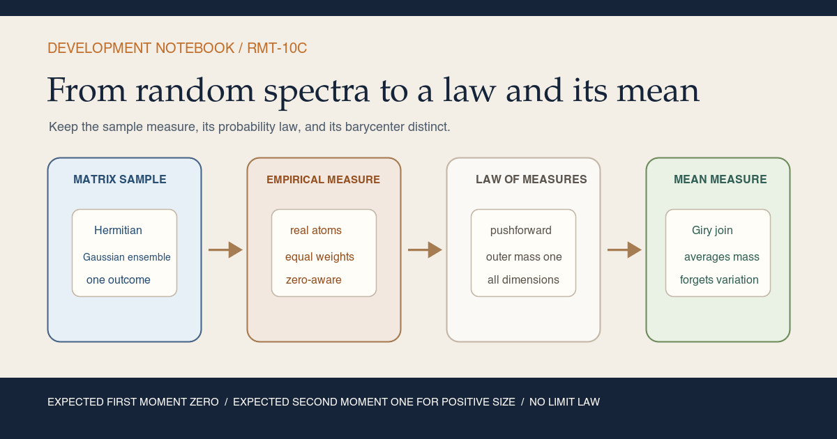
The central lesson is a type ladder. Let \(H\) be one intrinsic Hermitian matrix of size \(n\). RMT-10A assigns it the empirical spectral measure
\[ \mu_H=\frac1n\sum_{i=0}^{n-1}\delta_{\lambda_i(H)} \]when \(n\) is positive, with multiplicity retained. The project deliberately sets \(\mu_H=0\) when \(n=0\).
Now sample \(H\) from the intrinsic finite-GUE law \(\gamma_n\). The map \(H\mapsto\mu_H\) is a random variable whose codomain happens to be a space of measures. Its law is
\[ \mathcal L_n=(H\mapsto\mu_H)_*\gamma_n. \]Thus \(\mathcal L_n\) is not a measure on eigenvalue locations. It is a measure on possible measures on eigenvalue locations.
Finally, the barycenter averages those output measures:
\[ \overline\mu_n=\operatorname{join}(\mathcal L_n). \]This returns to a measure on \(\mathbb R\). On a measurable set \(S\), the Giry join is characterized by
\[ \overline\mu_n(S)=\int \mu(S)\,d\mathcal L_n(\mu). \]The right side averages how much mass each sampled spectral measure assigns to \(S\).
| Mathematical object | Lean shape | Where it lives |
|---|---|---|
| Matrix sample \(H\) | HermitianEuclidean n | Intrinsic Hermitian Euclidean space |
| Sample empirical measure \(\mu_H\) | Measure ℝ | Measures on the real line |
| Spectral law \(\mathcal L_n\) | Measure (Measure ℝ) | Measures on the space of measures |
| Mean empirical measure \(\overline\mu_n\) | Measure ℝ | Back on the real line |
flowchart LR
  H["one intrinsic Hermitian matrix"] --> M["one empirical spectral measure"]
  G["intrinsic finite GUE law"] --> P["push forward by the measurable spectrum map"]
  M --> P
  P --> L["probability law over measures"]
  L --> J["Giry join averages the random measures"]
  J --> B["mean empirical measure on the real line"]
Figure. The first arrow changes one matrix into one finite atomic measure. Pushforward remembers the full sample-to-sample distribution of those measures. Giry join then averages that distribution and discards its higher-order variability. The final measure is not the same object as the law over measures.
This ladder is not bureaucracy. A law retains fluctuations among spectra. A barycenter does not. Two ensembles can have the same mean empirical measure and different distributions of gaps, extreme eigenvalues, or linear statistics. RMT-10C names both objects so later work cannot silently substitute one for the other.
Moments of one realized spectrum
The first public declaration is
RandomMatrix.empiricalSpectralMoment. For a natural exponent
\(k\), it defines
The codomain is complex because it aligns with the existing complex trace-power observable. Every eigenvalue is real, so these particular values are real inside \(\mathbb C\), but the module does not add a separate theorem expressing that reality.
For positive dimension, expanding the atomic measure gives
\[ m_k(H)=\frac1n\sum_{i=0}^{n-1}\lambda_i(H)^k. \]RMT-10C exports only the cases needed to consume the checked trace integrals:
\[ m_1(H)=((n:\mathbb R)^{-1}:\mathbb C)\operatorname{Tr}(H), \]and
\[ m_2(H)=((n:\mathbb R)^{-1}:\mathbb C)\operatorname{Tr}(H^2). \]The Lean proofs do not reprove the spectral theorem. They unfold the empirical measure as a scalar multiple of the counting measure, move that scalar through the integral, and invoke RMT-10A:
integral_complex_ofReal_spectralCountingMeasureturns the first counting-measure integral into the matrix trace;integral_sq_complex_ofReal_spectralCountingMeasureturns the second into the trace of the square.
Those predecessor identities ultimately sit on Mathlib’s finite Hermitian spectral API (Mathlib Hermitian spectra).
The public theorems
RandomMatrix.empiricalSpectralMoment_one and
RandomMatrix.empiricalSpectralMoment_two are stated for every
natural dimension. At \(n=0\), both right sides contain a total field inverse
of zero, which is zero, and the zero matrix has zero trace. The equalities
therefore remain exact without an informal division by zero.
The zero-dimensional moment policy
RandomMatrix.empiricalSpectralMoment_zero is stronger than the
first two formulas. It proves that every exponent gives zero when the matrix
dimension is zero:
The reason is measure-theoretic, not a convention about \(0^0\). The zero-dimensional empirical spectral measure is the zero measure, and every integral against the zero measure is zero. In particular, the zeroth moment is zero at dimension zero, rather than the mass-one value familiar from a probability measure.
A probability law over raw measures
The definition GUE.empiricalSpectralLaw is the exact pushforward
where \(\gamma_n=\operatorname{GUE.intrinsicLaw}(n)\). RMT-10B supplied ordinary measurability of the map, so the definition carries no analytic hypothesis.
Its codomain is Measure (Measure ℝ). The inner
Measure ℝ is intentionally raw. It includes both mass-one
measures from positive dimensions and the zero measure selected at dimension
zero.
The instance
GUE.instIsProbabilityMeasureEmpiricalSpectralLaw says that
\(\mathcal L_n\) has total outer mass one for every \(n\). Pushforward preserves
the total mass of the intrinsic GUE probability law. This statement does not
say that every point in the support of \(\mathcal L_n\) is itself a probability
measure.
That distinction is clearest at dimension zero:
\[ \mathcal L_0=\delta_0. \]The Dirac measure \(\delta_0\) is an outer probability measure concentrated at the zero measure. Its sampled value \(0:\operatorname{Measure}(\mathbb R)\) has total mass zero. Outer probability and inner probability are separate claims.
GUE.empiricalSpectralLawProbability merely bundles this
all-dimensional outer result:
It changes the Lean type so probability-law APIs can consume the object. It does not change the points from raw measures into probability measures.
A law whose values are probability measures
Positive dimension supports a stricter construction.
GUE.empiricalSpectralProbabilityLaw n samples a matrix of size
\(n+1\), applies the bundled map
empiricalSpectralProbability n, and returns
Now both levels are certified:
- the outer distribution has total mass one; and
- every value carries an inner total-mass-one proof in its type.
The successor index is not a cosmetic way to avoid a proof branch. No bundled
ProbabilityMeasure ℝ can represent the zero measure chosen at
dimension zero. The all-dimension raw law and the successor-only bundled law
are therefore both necessary.
The theorem
GUE.map_empiricalSpectralProbabilityLaw_coe proves that forgetting
the inner probability wrapper recovers
GUE.empiricalSpectralLaw (n + 1). Its proof composes two
measurable maps:
- a matrix becomes a bundled empirical probability measure;
- subtype coercion forgets the bundle and returns the underlying raw measure.
Measure.map_map collapses the two pushforwards. The composition is
definitionally the raw empirical spectral measure. This theorem is an exact
compatibility bridge, not a claim that the zero-dimensional raw law can be
upgraded.
| Name | Outer package | Inner values | Dimensions |
|---|---|---|---|
empiricalSpectralLaw | Raw Measure, with a probability instance | Raw measures | All \(n\) |
empiricalSpectralLawProbability | Bundled ProbabilityMeasure | Raw measures | All \(n\) |
empiricalSpectralProbabilityLaw | Bundled ProbabilityMeasure | Bundled probability measures | Sizes \(n+1\) |
The similar names encode genuinely different types. Reading only their English glosses is risky. When debugging downstream Lean code, inspect the complete codomain first.
Intrinsic and ambient laws agree
The spectral law is defined using GUE.intrinsicLaw, whose samples
are Hermitian by type. Existing applications may instead start from
GUE.matrixLaw on the full ambient complex matrix space. RMT-10B
defined a total observable
ambientEmpiricalSpectralMeasure n: it recovers the intrinsic
matrix when the input is Hermitian and otherwise uses the project’s zero
fallback.
GUE.empiricalSpectralLaw_eq_map_matrixLaw_ambient proves
The proof is a one-line orientation of RMT-10B’s unconditional pushforward bridge. It shows that the newly named law is compatible with both established GUE presentations.
The theorem does not say the ambient fallback is a spectral theory for non-Hermitian matrices. The ambient GUE law gives the Hermitian locus full measure, so the fallback has no effect on the pushforward law. Off that almost-sure support it remains a totalization device.
Dimension zero, audited end to end
The dimension-zero branch is visible at every layer:
| Layer | Checked value at \(n=0\) | Reason |
|---|---|---|
| Intrinsic empirical measure | Zero measure | No eigenvalue indices and explicit zero-aware normalization |
| Any sample spectral moment | Zero | Integral against the zero measure |
| Spectral law | Dirac at the zero measure | Pushforward of the zero-dimensional intrinsic Dirac law |
| Outer law mass | One | A Dirac measure is a probability measure |
| Probability-valued spectral law | Not constructed | The inner zero measure is not a probability measure |
| Mean empirical measure | Zero measure | Giry join of a Dirac mass at zero |
| Expected first moment | Zero | Centered trace identity, also the sample zero theorem |
| Expected second moment | Zero | Total expression \(0^{-1}0=0\) in the field |
The theorem GUE.empiricalSpectralLaw_zero proves the Dirac row.
It maps the zero-dimensional intrinsic Dirac law through the measurable
empirical-measure map and simplifies the unique output to the zero measure.
The theorem GUE.meanEmpiricalSpectralMeasure_zero then rewrites
the barycenter definition, substitutes the Dirac law, and simplifies its join.
These are not merely consequences left for a reader. They freeze the boundary
policy into named rewrite rules for future modules.
There are two inverse conventions to keep separate. The raw empirical measure
uses an extended-nonnegative scalar. In that type,
\((0:\mathbb R_{\ge0}^{\infty})^{-1}=\infty\), while the empty counting measure
is zero, and the checked measure simplification is \(\infty\cdot0=0\).
The sample trace formulas instead expose the real inverse after
ENNReal.toReal; the real value \(0^{-1}\) is zero. Saying only
“the reciprocal is zero” would conflate those two stages.
Averaging a law of measures
GUE.meanEmpiricalSpectralMeasure is defined by
Mathlib’s Giry join flattens a measure of measures into a measure. For a measurable set \(S\), its evaluation theorem reads as the nonnegative integral of \(\mu(S)\) over the outer law. This is the precise sense in which the construction is the mean or barycenter of the random empirical measure (Mathlib Giry monad).
At positive dimension, every inner measure has total mass one. The theorem
GUE.meanEmpiricalSpectralMeasure_succ_isProbability proves that
the barycenter also has total mass one. Its proof uses
isProbabilityMeasure_join, whose key premise is that the outer law
lands almost everywhere in the measurable set of probability measures.
The proof establishes that premise under the pushforward by moving the
almost-everywhere statement back to intrinsic matrices. There the pointwise
theorem empiricalSpectralMeasure_succ_isProbability applies to
every sample. This sequence records the real probability logic:
- each successor-dimensional sample measure is a probability measure;
- the property is measurable in the Giry space;
- therefore the pushforward law is almost surely supported on probability measures;
- joining an outer probability law with probability-valued support preserves total mass one.
The bundled type, measurable support set, and join probability theorem are documented together in Mathlib’s probability-measure API.
RMT-10C does not prove an equation identifying the complex moments of \(\overline\mu_n\) with the expected sample moments below. Such an identity is mathematically natural but requires the relevant integration-through-join argument and integrability hypotheses in the exact complex-valued form. The module keeps its claims at the level actually checked.
Transporting integrability from ambient matrices
The private helper GUE.ambientTracePower specializes the existing
random-matrix observable to the identity sample map:
It gives the longer polymorphic expression a stable local name. This is the module’s only private declaration.
RMT-09 already proves that ambient trace powers one and two are Bochner
integrable under GUE.matrixLaw n. RMT-10C needs integrability of
the corresponding empirical spectral moment under
GUE.intrinsicLaw n. The bridge is the checked law identity
For exponent one, GUE.integrable_empiricalSpectralMoment_one
follows this proof spine:
- import
integrable_tracePower_one nunder the ambient law; - rewrite the ambient law as the pushforward of the intrinsic law;
- use
integrable_map_measureto transport integrability toambientTracePower n 1 ∘ hermitianToMatrix; - multiply by the constant reciprocal dimension;
- use
empiricalSpectralMoment_oneto identify the scaled composition with the desired sample moment.
The exponent-two theorem
GUE.integrable_empiricalSpectralMoment_two has the same
architecture with RMT-09’s second trace-power integrability.
This is not a free consequence of finite dimension. The sample space of matrices is unbounded, and a continuous polynomial observable need not be integrable under an arbitrary probability measure. Gaussian moment control, already established by RMT-09, supplies the finiteness.
Dimension zero gets a more general theorem:
GUE.integrable_empiricalSpectralMoment_zero k covers every
exponent. The function is pointwise zero by
empiricalSpectralMoment_zero, so it rewrites to the integrable
zero function. The companion
GUE.integral_empiricalSpectralMoment_zero k evaluates its
integral as zero.
Two transport lemmas with different jobs
integrable_map_measure transfers the finiteness property between a
function on the target of a pushforward and its composition on the source.
integral_map evaluates the integral after that transport. The
first prevents a totalized Bochner integral from hiding nonintegrability. The
second changes variables only after its measurability premise is supplied.
The module invokes both explicitly. This keeps expectation theorems from becoming bare equalities whose finiteness status is invisible. The underlying change-of-variables and Banach-valued integral interfaces are documented in Mathlib’s Bochner integration API.
The expected first moment is zero
GUE.integral_empiricalSpectralMoment_one n proves
for every natural dimension. Its calculation has four transparent steps:
\[ \begin{aligned} \int m_1(H)\,d\gamma_n(H) &= \int c_n\operatorname{Tr}(H)\,d\gamma_n(H)\\ &= c_n\int\operatorname{Tr}(H)\,d\gamma_n(H)\\ &= c_n\int\operatorname{Tr}(A)\,d\operatorname{matrixLaw}(n)(A)\\ &=c_n\cdot0=0, \end{aligned} \]where \(c_n=((n:\mathbb R)^{-1}:\mathbb C)\).
The first equality is the sample trace identity. The second pulls a constant
through the Bochner integral. The third is
integral_map along hermitianToMatrix. The fourth uses
RMT-09’s exact centered trace integral.
The statement is a first moment of the random empirical measure, averaged over the intrinsic matrix law. It does not prove that each sample has zero first moment. Individual matrices generally have nonzero trace. Centering is an ensemble expectation.
Why the second expected moment is one
The all-dimensional theorem
GUE.integral_empiricalSpectralMoment_two n proves
The proof mirrors the first-moment calculation but ends with RMT-09’s exact identity
\[ \int\operatorname{Tr}(A^2)\, d\operatorname{matrixLaw}(n)(A)=n. \]Why retain the unsimplified product? It is the exact theorem for all natural dimensions. In Lean’s fields, \(0^{-1}=0\), so at \(n=0\) the right side is zero. For positive \(n\), reciprocal cancellation is valid and the value is one.
GUE.integral_empiricalSpectralMoment_two_succ n states that
positive-dimensional corollary directly:
The proof rewrites with the all-dimensional theorem, coerces the arithmetic, and invokes inverse cancellation with positivity of \(n+1\).
This value is the finite normalization certificate. RMT-09 proved \(\mathbb E\operatorname{Tr}(H^2)=n\) for the Wigner-scaled ensemble. Dividing the spectral sum by the number of eigenvalues gives average squared spectral location one. It is consistent with an order-one spectral scale, but it does not identify the distribution of those locations.
Physics reading: density of states and ensemble disorder
Read \(H\) as a finite Hamiltonian after a choice of energy units. Its eigenvalues are the allowed energies, repeated by degeneracy. The sample empirical measure
\[ \mu_H=\frac1n\sum_i\delta_{\lambda_i(H)} \]is the normalized finite density of states: it reports the fraction of energy levels in each measurable region of the real line.
The law \(\mathcal L_n\) answers a different physical question. If the Hamiltonian is drawn from an ensemble, how does the entire density-of-states measure fluctuate from one realization to another? An event in this law can describe a set of possible empirical measures. The barycenter \(\overline\mu_n\) instead answers the ensemble-averaged density-of-states question. It gives expected level mass in an energy window, but it cannot say whether individual samples fluctuate coherently around that average.
This separation matters in disordered systems and quantum chaos. A mean density can be smooth even though each finite sample is atomic. It can also be identical for two ensembles with different level correlations. Repulsion, gap distributions, and extreme-level fluctuations require more than the barycenter. The law-over-measures layer is closer to those questions, though RMT-10C does not yet formalize their observables.
The first sample moment is the energy centroid:
\[ m_1(H)=\frac1n\operatorname{Tr}(H). \]Its ensemble mean zero says that the GUE energy cloud is centered under the chosen normalization. It does not say each Hamiltonian is traceless. The second sample moment is the mean squared energy:
\[ m_2(H)=\frac1n\operatorname{Tr}(H^2). \]Its positive-dimensional ensemble mean one calibrates the global quadratic energy scale. It does not bound every energy by one, determine the spectral edge, or identify a density.
Unitary conjugation is a change of orthonormal basis for the finite Hilbert space. Earlier modules prove both unitary invariance of the GUE matrix law and unitary invariance of the ordered spectrum. Those ingredients explain why the spectral constructions are physically basis-independent. RMT-10C consumes the resulting intrinsic law and spectrum map, but it does not export a new named unitary-invariance theorem for \(\mathcal L_n\).
The complete declaration map
The module exports twenty-one declarations and keeps one helper private. The tables follow source order and preserve namespace qualification.
Public API: sample spectral moments
| Declaration | Exact role | Proof engine |
|---|---|---|
RandomMatrix.empiricalSpectralMoment | Defines the \(k\)-th complex moment of one zero-aware empirical spectral measure | Bochner integral of the complex-coerced power |
RandomMatrix.empiricalSpectralMoment_zero | Proves every exponent gives zero in dimension zero | Empirical measure is zero, then integral against zero |
RandomMatrix.empiricalSpectralMoment_one | Identifies the first sample moment with reciprocal-dimension trace | Unfold normalization and apply the counting-measure trace integral |
RandomMatrix.empiricalSpectralMoment_two | Identifies the second sample moment with reciprocal-dimension trace square | Unfold normalization and apply the counting-measure square integral |
Public API: laws and barycenter
| Declaration | Exact role | Proof engine |
|---|---|---|
GUE.empiricalSpectralLaw | Defines the intrinsic finite-GUE pushforward law on raw empirical measures | intrinsicLaw.map empiricalSpectralMeasure |
GUE.instIsProbabilityMeasureEmpiricalSpectralLaw | Gives the raw spectral law outer mass one in every dimension | Probability preservation under measurable pushforward |
GUE.empiricalSpectralLawProbability | Bundles the all-dimensional outer law as a probability measure on raw measures | The preceding probability instance |
GUE.empiricalSpectralProbabilityLaw | Defines the successor-dimensional outer probability law valued in bundled probability measures | Pushforward through empiricalSpectralProbability |
GUE.map_empiricalSpectralProbabilityLaw_coe | Shows that forgetting inner probability wrappers recovers the raw successor law | Measurable subtype coercion and Measure.map_map |
GUE.empiricalSpectralLaw_eq_map_matrixLaw_ambient | Identifies intrinsic and ambient presentations of the named spectral law | RMT-10B’s unconditional pushforward bridge |
GUE.empiricalSpectralLaw_zero | Computes the dimension-zero law as a Dirac mass at the zero measure | Map the intrinsic zero-dimensional Dirac law |
GUE.meanEmpiricalSpectralMeasure | Defines the barycenter of the raw spectral law | Giry Measure.join |
GUE.meanEmpiricalSpectralMeasure_zero | Computes the zero-dimensional barycenter as the zero measure | Join the Dirac law at zero |
GUE.meanEmpiricalSpectralMeasure_succ_isProbability | Proves the positive-dimensional barycenter has total mass one | Almost-sure probability-valued support and isProbabilityMeasure_join |
Public API: integrability and exact expectations
| Declaration | Exact role | Proof engine |
|---|---|---|
GUE.integrable_empiricalSpectralMoment_zero | Proves every exponent integrable in dimension zero | Rewrite the observable to the zero function |
GUE.integral_empiricalSpectralMoment_zero | Evaluates every dimension-zero expected spectral moment as zero | Pointwise zero and integral_eq_zero_of_ae |
GUE.integrable_empiricalSpectralMoment_one | Proves first sample moments integrable under every intrinsic finite-GUE law | Transport ambient trace integrability and multiply by reciprocal dimension |
GUE.integral_empiricalSpectralMoment_one | Evaluates the expected first sample moment as zero in every dimension | Sample trace formula, integral_map, and RMT-09 trace centering |
GUE.integrable_empiricalSpectralMoment_two | Proves second sample moments integrable under every intrinsic finite-GUE law | Transport ambient trace-square integrability and scale |
GUE.integral_empiricalSpectralMoment_two | Evaluates the all-dimensional expectation as \(n^{-1}n\) | Sample trace-square formula, law transport, and RMT-09 second trace integral |
GUE.integral_empiricalSpectralMoment_two_succ | Simplifies the positive-dimensional expected second moment to one | All-dimensional identity plus nonzero inverse cancellation |
Private helper
| Declaration | Proof job |
|---|---|
GUE.ambientTracePower | Names RandomMatrix.tracePower id k on the ambient \(n\)-by-\(n\) complex matrix carrier so transport calculations remain readable |
The public dependency spine is deliberate. Sample identities come first, then law packaging and barycenters, then integrability and expectation. Downstream files can import a named spectral law without inheriting a private proof representation for trace transport.
Lean proof engineering
Why define the raw law before the bundled law?
The zero-aware observable is total in every dimension and naturally lands in
Measure ℝ. Defining its raw pushforward preserves that uniform
interface. Probability structure is then layered on: an outer instance in all
dimensions, an outer bundle in all dimensions, and an inner probability-valued
bundle only for successors.
Why does the outer law use the intrinsic presentation?
The intrinsic sample space makes Hermiticity true by type and avoids carrying an almost-everywhere support proof into every later theorem. The ambient presentation remains available through a named equality, so matrix-law users lose nothing.
Why use Giry join instead of an informal expectation symbol?
The output of the random variable is itself a measure. Giry join is Mathlib’s canonical measurable flattening operation. It supplies a set-evaluation semantics and composes with the existing measure-valued measurable structure. An overloaded scalar expectation symbol would hide both the codomain and the required measurability.
Why prove integrability again after RMT-09?
RMT-09’s observable and measure live on the ambient matrix carrier. RMT-10C’s observable and measure live on the intrinsic Hermitian carrier. Their values are pointwise related, and their laws are connected, but Lean still needs the explicit transport theorem to move the integrability fact across that bridge.
Why keep the all-dimensional second expectation unsimplified?
The expression \(n^{-1}n\) displays the exact normalization and handles zero without a false cancellation. The successor theorem performs cancellation only where positivity proves the denominator nonzero.
Why is there no theorem about the barycenter’s second moment?
The module proves sample-moment integrability under the matrix law and defines the measure barycenter. Connecting a complex Bochner moment of the join to an iterated integral is a further theorem. It should be proved with the precise integrability and Giry interfaces, not asserted because the notation looks like expectation.
How to run the checked source
Compile the module directly with every warning promoted to an error:
source "$HOME/.elan/env"
cd formalization
lake env lean -DwarningAsError=true \
  NonlinearDynamics/Random/RandomMatrices/GaussianUnitaryEnsembleSpectrum.lean
Build the complete Lean library:
source "$HOME/.elan/env"
cd formalization
lake build
From the repository root, check the public teaching content:
make content-hygiene
make site-check
This complete Lean snippet checks every public declaration:
import NonlinearDynamics.Random.RandomMatrices.GaussianUnitaryEnsembleSpectrum

open Matrix MeasureTheory
open scoped ENNReal Matrix
open NonlinearDynamics.Random

#check RandomMatrix.empiricalSpectralMoment
#check RandomMatrix.empiricalSpectralMoment_zero
#check RandomMatrix.empiricalSpectralMoment_one
#check RandomMatrix.empiricalSpectralMoment_two
#check GUE.empiricalSpectralLaw
#check GUE.instIsProbabilityMeasureEmpiricalSpectralLaw
#check GUE.empiricalSpectralLawProbability
#check GUE.empiricalSpectralProbabilityLaw
#check GUE.map_empiricalSpectralProbabilityLaw_coe
#check GUE.empiricalSpectralLaw_eq_map_matrixLaw_ambient
#check GUE.empiricalSpectralLaw_zero
#check GUE.meanEmpiricalSpectralMeasure
#check GUE.meanEmpiricalSpectralMeasure_zero
#check GUE.meanEmpiricalSpectralMeasure_succ_isProbability
#check GUE.integrable_empiricalSpectralMoment_zero
#check GUE.integral_empiricalSpectralMoment_zero
#check GUE.integrable_empiricalSpectralMoment_one
#check GUE.integral_empiricalSpectralMoment_one
#check GUE.integrable_empiricalSpectralMoment_two
#check GUE.integral_empiricalSpectralMoment_two
#check GUE.integral_empiricalSpectralMoment_two_succ
Save the snippet inside formalization and run
lake env lean path/to/Scratch.lean. The private helper is
intentionally absent from this import-level API audit.
Useful local Mathlib reconnaissance:
rg -n "def join|join_apply|isProbabilityMeasure_join" \
  formalization/.lake/packages/mathlib/Mathlib/MeasureTheory/Measure

rg -n "integrable_map_measure|theorem integral_map" \
  formalization/.lake/packages/mathlib/Mathlib/MeasureTheory/Integral

rg -n "measurableSet_isProbabilityMeasure" \
  formalization/.lake/packages/mathlib/Mathlib/MeasureTheory/Measure
The pinned local Mathlib 4.32.0 release source is the exact API authority. Online documentation is a navigational aid, not a replacement for compiling against the selected checkout.
Common failure modes
Calling a sample empirical measure its law
empiricalSpectralMeasure H has type Measure ℝ.
empiricalSpectralLaw n has type
Measure (Measure ℝ). Confusing them removes one probability layer
and turns statements about ensemble variability into statements about one
matrix.
Calling the barycenter the law
meanEmpiricalSpectralMeasure n returns to
Measure ℝ. It averages set masses and forgets the distribution
among sample measures. It cannot answer fluctuation questions that the law
retains.
Assuming outer probability implies inner probability
At dimension zero, the spectral law is a probability measure concentrated at
the zero measure. The zero measure is not itself a probability measure. The
outer instance does not justify constructing
ProbabilityMeasure ℝ values.
Swapping the two probability-law wrappers
empiricalSpectralLawProbability bundles only the outer law.
empiricalSpectralProbabilityLaw bundles outer and inner
probability and therefore uses size \(n+1\). Inspect the nested codomain rather
than relying on their similar names.
Canceling dimension at zero
The all-dimensional second expectation is \(n^{-1}n\), not unconditionally one. Cancellation requires \(n\ne0\). The successor theorem supplies that proof and only then concludes one.
Giving the wrong value to an extended-nonnegative inverse
The scalar in empiricalSpectralMeasure is extended nonnegative.
Its inverse at zero is infinity, not zero. The measure is still zero because
the counting measure is empty and infinity scales the zero measure to zero.
Only after ENNReal.toReal does the normalization appearing in the
complex trace formula become real zero.
Treating integrability as automatic
Finite matrix dimension does not make an unbounded polynomial observable integrable under every law. The proof imports Gaussian trace-moment integrability and transports it across the intrinsic-to-ambient pushforward.
Reversing integral_map
The source measure is intrinsic and the map is
hermitianToMatrix. After mapping, the integral is under the
ambient matrix law. Reversing that direction produces the wrong composition
and mismatched carrier types.
Reading the zero policy as a hidden probability completion
The dimension-zero empirical measure is exactly zero. No dummy eigenvalue is inserted, and no arbitrary probability distribution is selected to fill the empty spectrum.
Equating expected sample moments with barycenter moments without proof
The module evaluates integrals of empiricalSpectralMoment under
the intrinsic law. It does not export the corresponding integral against
meanEmpiricalSpectralMeasure. Interchanging the Giry join and a
complex-valued integral remains a separate formal obligation.
Inferring a density from a named law
A probability law on the measurable space of measures need not admit a density with respect to any convenient reference measure. Naming the pushforward and proving its mass do not produce a finite-dimensional eigenvalue density.
Strict nonclaims
RMT-10C does not prove:
- a joint density for the ordered GUE eigenvalues;
- a matrix-to-eigenvalue change-of-variables theorem;
- a Vandermonde determinant or Jacobian factor;
- absolute continuity of the empirical spectral law;
- a closed-form finite-dimensional mean spectral density;
- a formula for the moments of
GUE.meanEmpiricalSpectralMeasure; - equality between a barycenter moment and the expected sample moment;
- integrability or expectation of empirical spectral moments above degree two;
- Wick expansion, pairing enumeration, or Catalan moment formulas;
- variance, covariance, or concentration of spectral linear statistics;
- largest-eigenvalue or smallest-eigenvalue distributions;
- level spacing, repulsion, unfolding, or local correlation functions;
- finite-\(n\) determinantal kernels or Hermite-polynomial formulas;
- compact support of a finite-GUE sample or its mean measure;
- convergence in probability, almost surely, weakly, or in Wasserstein distance;
- a semicircle law or a rate of convergence to one;
- edge scaling, Tracy-Widom behavior, sine-kernel statistics, or universality;
- non-Hermitian spectral laws;
- a numerical eigensolver or floating-point error theorem; or
- a quantum-chaos diagnostic.
The exact output is a finite measurable law-and-moment layer. The first two normalized expectations are normalization checks, not a reconstruction of a distribution.
Exercises with solutions
Exercise 1: read the type ladder
What are the codomains of empiricalSpectralMeasure,
empiricalSpectralLaw, and
meanEmpiricalSpectralMeasure?
Solution. They are Measure ℝ,
Measure (Measure ℝ), and Measure ℝ, respectively.
The repeated first and third codomains do not make those objects equal: one is
a sample output, the other is an ensemble barycenter.
Exercise 2: audit outer and inner mass
Why can \(\delta_0\) be a probability law when its point \(0\) is not a probability measure on \(\mathbb R\)?
Solution. The outer Dirac law assigns mass one to the singleton containing the zero measure. The inner zero measure assigns mass zero to the real line. The masses belong to different measurable spaces.
Exercise 3: expand a sample moment
For a positive-dimensional Hermitian matrix with eigenvalues \(\lambda_0,\ldots,\lambda_{n-1}\), what is \(m_2(H)\)?
Solution.
\[ m_2(H)=\frac1n\sum_i\lambda_i^2 =\frac1n\operatorname{Tr}(H^2). \]Multiplicity is retained by the indexed sum.
Exercise 4: handle the empty spectrum
What is \(m_0(H)\) when \(H\) has dimension zero?
Solution. It is zero. The integral is against the zero empirical measure. The answer is not obtained by evaluating \(0^0\).
Exercise 5: distinguish two bundles
Which definition can be used in dimension zero:
empiricalSpectralLawProbability or
empiricalSpectralProbabilityLaw?
Solution. The first. It bundles the outer law on raw measures. The second requires positive dimension because its inner values are bundled probability measures.
Exercise 6: evaluate the barycenter on a set
What does \(\overline\mu_n(S)\) mean for measurable \(S\)?
Solution. It is the outer-law average of \(\mu(S)\) over sampled empirical measures \(\mu\). It is expected spectral mass in \(S\), not the probability of one particular empirical measure.
Exercise 7: transport integrability
Why is the equality
matrixLaw_eq_map_hermitianToMatrix_intrinsicLaw useful?
Solution. It rewrites the ambient measure as a pushforward. Mathlib’s
integrable_map_measure then transfers RMT-09’s ambient
trace-power integrability to the trace-power composition on intrinsic
Hermitian samples.
Exercise 8: compute the first expectation
If \(\mathbb E\operatorname{Tr}(H)=0\), what is \(\mathbb E m_1(H)\)?
Solution. It is the reciprocal-dimension constant times zero, hence zero. The dimension-zero case also agrees because the sample moment is identically zero.
Exercise 9: simplify the second expectation
Why is \(\mathbb E m_2(H)=1\) stated only for dimensions \(n+1\)?
Solution. The all-dimensional value is \(n^{-1}n\). At zero it is zero under Lean’s total inverse. At a successor, positivity permits reciprocal cancellation and yields one.
Exercise 10: test the claim boundary
Do mean zero and second moment one determine the semicircle law?
Solution. No. Infinitely many probability distributions share those two moments. A semicircle theorem needs control of a determining family of observables together with an asymptotic convergence argument.
Exercise 11: compare law and barycenter
Could two spectral laws have the same barycenter?
Solution. Yes. Averages can agree while sample-to-sample fluctuations differ. The law over measures retains those differences; the joined measure does not.
Exercise 12: identify the unproved interchange
What additional bridge would connect the checked expected sample second moment to a second moment of the mean empirical measure?
Solution. One needs a theorem moving the complex function \(x\mapsto x^2\) through the Giry join, with the required measurability and integrability. RMT-10C does not export that theorem.
The next ridge
RMT-10C completes the first finite-GUE spectral-law interface. A downstream module can now refer to a named probability law over empirical measures, choose the stricter positive-dimensional probability-valued package when needed, and consume exact normalized moments without rebuilding trace transport.
Its immediate successor, Ordered Finite Matrix Products in Lean, returns to the dependency-ordered deterministic branch. It fixes the newest-factor-left time convention, proves shifted splitting and chronological vector action, and establishes finite-time product and power bounds in the maximum-row-sum operator norm before measurable random products and cocycles.
Within spectral theory, later self-contained milestones may add higher finite trace moments, a rigorously derived finite-dimensional eigenvalue density, or an integration-through-barycenter theorem. Any semicircle law must remain a separate asymptotic development with an explicit convergence mode and enough moment or transform control to justify the limit.
References
The links below were checked on 2026-07-21. The pinned local Mathlib 4.32.0 checkout remains the exact API authority for the Lean proof.
Alice Guionnet. “Rare Events in Random Matrix Theory”, Proceedings of the International Congress of Mathematicians 2022, volume 2, pages 1008-1052. The survey records the classical Wigner-scaled GUE normalization and the relation between normalized trace powers and empirical spectral moments. It supplies context, not the checked law packaging or integrability transport.
Mathlib contributors.
Mathlib 4.32.0 release,
2026. This is the dependency release selected by
formalization/lakefile.toml.
Mathlib contributors.
The Giry monad,
Mathlib 4 documentation. This official page defines Measure.join
and its measurable-set evaluation, the formal barycenter operation used by
meanEmpiricalSpectralMeasure.
Mathlib contributors.
Probability measures,
Mathlib 4 documentation. This official page defines the bundled
ProbabilityMeasure type, the measurable set of probability
measures inside a measure space, and probability preservation under Giry join.
Mathlib contributors.
Bochner integration,
Mathlib 4 documentation. This official page supplies
integral_map, constant multiplication, and the Banach-valued
integral interfaces used in the exact expectation proofs.
Mathlib contributors. Hermitian matrix spectra, Mathlib 4 documentation. This official page documents the finite Hermitian spectral theorem and eigenvalue-sum identities beneath the project’s ordered spectral measure.