This is the proof-to-prose companion for
formalization/NonlinearDynamics/Random/RandomCocycles/FiniteHopfMaximal.lean.
It covers all twenty-five documented public declarations in exact source order,
the private integral-cancellation helper in its actual position, and all eleven
anonymous compiled boundary probes.
Its immediate predecessor is Convergence Without Existence: Birkhoff Events and Ergodic Rigidity in Lean. That chapter built a measurable convergence event and proved it invariant, but did not prove that any point enters it. The present finite maximal lemma is the first analytic estimate aimed at the missing existence direction. It still does not cross that gap by itself.
The underlying finite sums reuse the Birkhoff sum . The distinction between raw measure preservation, probability normalization, and ergodicity remains the one developed in the ergodic probability base entry. A later pointwise theorem would return to the Birkhoff convergence event . The stable definition introduced by this milestone is the finite maximal ergodic inequality . The parallel textbook treatment is Finite Maximal Ergodic Inequalities: From Orbit Maxima to Threshold Events.
Choose a route up
| Route | Begin | Destination |
|---|---|---|
| First encounter | Why watch the largest partial sum? | See why a running maximum detects a positive excursion that the terminal sum can miss |
| Historical route | Four sources, four different theorem shapes | Separate Yosida–Kakutani, Hopf, Garsia, and Keane–Petersen from the exact Lean slice |
| Finite-order route | Build a maximum that remembers time zero | Understand Finset.sup’, nonnegativity, monotonicity, and edge horizons |
| Event route | Strict positivity keeps the event informative | Derive the positive-index witness and nested events |
| Proof route | Peel a positive maximizing index | Prove the central pointwise indicator inequality |
| Measure route | Integrate and cancel the shifted maximum | Reach the finite Hopf-style lemma without probability or invertibility |
| Threshold route | Center first, divide last | Reach finite average-exceedance and weak measure estimates |
| API route | The complete source-order tour | Audit every public declaration and the private helper |
| Boundary route | Eleven probes test the theorem’s edges | Check zero, one, identity, infinite measure, noninvertibility, and failed preservation |
| Integrity route | The exact premise and nonclaim ledger | Prevent finite estimates from being narrated as asymptotic theorems |
Learning objectives
By the summit, a reader should be able to:
- define the finite running maximum of Birkhoff sums through a horizon;
- explain why the index set is nonempty for every natural horizon;
- explain why including time zero forces the maximum to be nonnegative;
- distinguish the running maximum from the positive part of the terminal sum;
- state why increasing the horizon can only increase the maximum;
- compute the maximum at horizons zero and one;
- separate ordinary measurability of the maximum from its integrability;
- explain how measure preservation propagates one-step integrability through finite sums;
- define the strict finite Hopf event;
- explain why a nonnegative event would be universal;
- turn strict event membership into a positive-time witness;
- explain why the witnessing index cannot be zero;
- choose an actual maximizing index from a finite supremum;
- peel a positive successor sum into the first value and a shifted sum;
- prove the pointwise inequality on the event;
- prove its zero-indicator branch off the event;
- combine both branches as one indicator inequality;
- distinguish measurable from null-measurable event interfaces;
- explain why integrability is enough for the main set integral;
- derive equality of shifted and unshifted maximal integrals from measure preservation;
- explain why this cancellation needs no inverse map;
- derive the nonnegative event integral;
- define average exceedance through the centered observable \(g-a\);
- prove that a centered positive sum is a positive-time average exceedance;
- identify exactly where finite total mass first enters;
- derive the threshold times measure lower bound for every real threshold;
- explain why replacing \(g\) by its positive part gives a uniform right side;
- identify exactly where positivity of the threshold first enters;
- read all eleven boundary probes as tests of the theorem’s quantifiers; and
- list the infinite-horizon, convergence, subadditive, and cocycle conclusions still absent.
Why watch the largest partial sum?
Take one orbit
\[ \omega,\quad T\omega,\quad T^2\omega,\quad\ldots \]and read a real observable along it. The finite sum \(S_k g(\omega)\) records the accumulated reading through time \(k-1\). A terminal sum at one chosen horizon can hide the path taken to reach it. For example, a sequence of readings may begin with a strong positive excursion and later fall below zero. The terminal sum then says nothing about the earlier excursion.
The running maximum remembers whether any prefix became positive:
\[ M_Ng(\omega)=\max\{S_0g(\omega),S_1g(\omega),\ldots,S_Ng(\omega)\}. \]This is not the positive part of \(S_N\). The positive part asks only for \(\max(S_N,0)\). The running maximum asks for the largest value among every prefix. Confusing those two objects destroys the proof. Garsia’s notation in the closest primary source denotes a running maximum; it must not be read as the positive part of the terminal sum (Garsia, 1965, p. 381).
The time-zero sum is deliberately included. Mathlib’s
birkhoffSum gives \(S_0=0\), so the running maximum is never
negative. This convention has two benefits. It avoids a separate empty-index
maximum at \(N=0\), and it makes the off-event branch exact: if the maximum is
not positive, then it must equal zero.
The price is equally important. The event must use strict positivity. Since \(M_N\ge0\) everywhere, the set where \(0\le M_N\) is always the entire state space. One of the compiled probes states exactly that universal-set identity.
A small orbit example
Suppose the first three readings are
\[ g(\omega)=-2,\qquad g(T\omega)=5,\qquad g(T^2\omega)=-10. \]The prefix sums at times zero through three are \(0,-2,3,-7\). The terminal sum is negative, and its positive part is zero. The running maximum is three, so the point belongs to the strict maximal event. The positive excursion is real finite-time information even though it does not survive to the terminal horizon.
This numerical illustration is not an empirical result and does not appear as a theorem. Its only job is to keep the two maximum conventions distinct.
Four sources, four different theorem shapes
The name “Hopf-style” records mathematical lineage without claiming that the Lean statement is a transcription of one historical theorem. The relevant sources differ in horizon, normalization, transformation assumptions, and proof architecture.
Yosida and Kakutani: the name and an early point-transformation theorem
Yosida and Kakutani’s 1939 paper states its setting on page 165: a one-to-one measure-preserving point transformation, with no assumption that the total measure is finite. The same page labels its second theorem as new and says that they will call it the “Maximal Ergodic Theorem” (Yosida and Kakutani, 1939, p. 165). Pages 166 and 167 develop a maximal-interval selection argument (open scan).
That paper is essential historical evidence, but it is not the literal source of the Lean proof. Its theorem is phrased using infinite-horizon average objects, its transformation is one-to-one, and its interval argument is not the finite running-maximum cancellation implemented here. RMT-23 drops injectivity and stops at a fixed horizon.
Hopf: broader operator lineage
Hopf’s 1954 article, The General Temporally Discrete Markoff Process, is the broader operator-theoretic source behind the later theorem name (Hopf, 1954). The journal record verifies the title, author, volume, issue, year, and page range 13–45. The available article-level archive did not provide a freely inspectable internal theorem page during this audit, so this chapter does not attach a theorem number or page-specific statement to Hopf. It cites the article for lineage only.
Garsia: the closest finite proof source
Garsia’s two-page 1965 note is the closest source for the formal architecture. On page 381 he considers a positive norm-nonincreasing linear operator on \(L^1\), defines \(S_0(f)=0\), defines finite partial sums, takes their running maximum through \(n\), and uses the strict set where that maximum is positive. His displayed theorem integrates \(f\) nonnegatively over that set. The basic pointwise step is the operator inequality saying that \(f\) dominates the running maximum minus its image under the operator (Garsia, 1965, p. 381).
RMT-23 specializes that operator picture to the Koopman operator associated with a point map. If \(U h=h\circ T\), then measure preservation makes \(U\) integral-preserving on integrable functions. The Lean inequality
\[ M_Ng-M_Ng\circ T\le\mathbf 1_{E_N(g)}g \]is the point-map version of Garsia’s core comparison. The Lean proof is still its own checked artifact: it works through Mathlib’s finite supremum, measurability, null-measurability, Bochner integral, and pushforward APIs.
Keane and Petersen: a later finite-to-infinite route
Keane and Petersen begin on a probability space with a possibly noninvertible measure-preserving transformation. On pages 248 and 249 they define finite maxima of averages, strict finite events, and then pass toward an infinite-horizon maximal theorem and a pointwise ergodic theorem (Keane and Petersen, 2006, pp. 248–249). Their proof organizes orbit segments into bounded strings; it is not the same finite integral-cancellation proof as RMT-23.
The source is valuable for what comes next. It shows one historical route from finite events toward an infinite theorem and pointwise convergence. RMT-23 formalizes only the finite estimate needed before such a passage can be audited. It does not import their limiting argument, bounded approximation, or dominated-convergence steps.
Lineage ledger
| Source | Transformation or operator | Horizon and event | Role here | Not silently imported |
|---|---|---|---|---|
| Yosida–Kakutani 1939 | One-to-one measure-preserving point map; total mass need not be finite | Infinite-horizon average formulation | Historical naming and early maximal-interval proof | Injectivity, their exact asymptotic statement, or their interval proof |
| Hopf 1954 | Broader temporally discrete Markov/operator setting | Article-level lineage | Source of the operator tradition | An unverified theorem number or internal page claim |
| Garsia 1965 | Positive norm-nonincreasing linear operator on \(L^1\) | Finite running partial-sum maximum and strict positive event | Closest pointwise and integral proof architecture | The full abstract operator theorem as a project API |
| Keane–Petersen 2006 | Possibly noninvertible measure-preserving map on a probability space | Finite average maxima followed by infinite limits | Guide to a later finite-to-infinite development | Probability, bounded approximation, dominated convergence, or pointwise convergence |
Build a maximum that remembers time zero
The first public declaration is the finite maximal function itself:
def finiteBirkhoffSumMax (T : Ω → Ω) (g : Ω → ℝ) (N : ℕ) : Ω → ℝ :=
  fun ω ↦
    (Finset.range (N + 1)).sup' Finset.nonempty_range_add_one
      (fun k ↦ birkhoffSum T g k ω)
Finset.range (N + 1) contains exactly the natural numbers strictly
below \(N+1\), hence the horizons zero through \(N\). The proof term
Finset.nonempty_range_add_one certifies that this set is nonempty.
That witness licenses Finset.sup’, a supremum over a known
nonempty finite set. There is no artificial default value from an
OrderBot instance.
The implementation follows the mathematical object directly. It does not convert the finite set into a list, sort the values, or choose an arbitrary sentinel. The pinned Mathlib finite-lattice API supplies induction, evaluation, strict-witness, and maximizing-index lemmas for exactly this construction (finite supremum API).
Every prefix lies below the maximum
birkhoffSum_le_finiteBirkhoffSumMax says that if \(k\le N\), then
The proof turns \(k\le N\) into membership in
Finset.range (N + 1), then applies Finset.le_sup’.
This lemma becomes the reusable comparison at time zero, under horizon
extension, and after peeling a positive maximizing index.
Time zero forces nonnegativity
finiteBirkhoffSumMax_nonneg specializes the preceding comparison
to \(k=0\). Since the zero-horizon Birkhoff sum is zero,
No measurability, measure, or dynamical assumption is involved. This is finite order algebra.
Larger horizons retain every earlier candidate
finiteBirkhoffSumMax_mono proves
The proof applies the finite-supremum attainment theorem to obtain an index at which its maximum is attained. That index lies below \(M\), hence below \(N\), so the universal prefix comparison bounds its value by the larger maximum. Finite attainment, not compactness or topology, does all the work.
The zero horizon is exact
finiteBirkhoffSumMax_zero is a simplification theorem:
At horizon zero, the index set contains only zero and the only Birkhoff sum is zero. This equality later makes the strict event empty without an integral argument.
Measurability and integrability are different gates
The pointwise maximum exists for every map and observable. Using it under an integral requires analytic evidence, and RMT-23 provides two deliberately different routes.
Ordinary measurability
measurable_finiteBirkhoffSumMax assumes ordinary measurability of
both \(T\) and \(g\). The preceding RMT-22 module proves that every finite
Birkhoff sum is measurable under those hypotheses. Mathlib’s
Finset.measurable_range_sup’’ then packages the finite pointwise
maximum as a measurable function
(measurable finite suprema).
This theorem is the clean route when the chosen representative of \(g\) is ordinarily measurable. It does not assume integrability, preservation, finite measure, probability, or ergodicity.
Integrability under preservation
integrable_finiteBirkhoffSumMax instead assumes
(hT : MeasurePreserving T μ μ) (hg : Integrable g μ)
for one arbitrary measure \(\mu\). The imported finite-sum theorem propagates
the integrability of \(g\) through every iterate and every finite sum. The new
proof uses Finset.sup’_induction: the pointwise supremum of two
integrable real functions is integrable, and each leaf Birkhoff sum is
integrable. Finally, Finset.sup’_apply aligns the supremum of
functions with its pointwise evaluation.
This route deliberately does not request ordinary measurability of \(g\).
Mathlib’s Integrable includes almost-everywhere strong
measurability and finite integral norm. That is enough for the null-measurable
event and indicator integral used by the main theorem.
Measure preservation carries measurability of \(T\), but it carries more than measurability: it makes every orbit shift preserve the source measure. That is why it supports finite-sum integrability and later integral cancellation.
What remains absent
Neither theorem assumes that \(\mu(\Omega)=1\). Neither assumes that total mass is finite. Neither assumes ergodicity or any mixing property. Integrability of one observable is not stationarity or independence. Finite integrability also does not imply convergence of normalized sums.
Strict positivity keeps the event informative
The next definition is
def finiteHopfEvent (T : Ω → Ω) (g : Ω → ℝ) (N : ℕ) : Set Ω :=
  { ω | 0 < finiteBirkhoffSumMax T g N ω }
The word finite matters twice. The maximum ranges over finitely many horizons, and the event records a positive excursion before one fixed cutoff. It is not an event defined by a supremum over all time.
Two event-regularity routes
measurableSet_finiteHopfEvent combines ordinary measurability of
the maximum with measurability of a strict real inequality. Its assumptions
are ordinary measurability of \(T\) and \(g\).
nullMeasurableSet_finiteHopfEvent_of_integrable is weaker in the
right direction for the main theorem. Measure preservation and integrability
make the maximal function almost-everywhere measurable, so its strict
positivity event is null-measurable. A null-measurable set may differ from an
ordinary measurable set on a null exception. That is sufficient for
indicators, restrictions, and set integrals modulo null sets.
The theorem does not manufacture an ordinarily measurable version of the raw event. It exposes exactly the regularity the integral proof consumes.
A positive event has a positive-time witness
mem_finiteHopfEvent_iff states
The forward proof turns positivity of the finite supremum into a member whose
value is positive using Finset.lt_sup’_iff. The candidate index is
at most \(N\). It cannot be zero, because \(S_0=0\) contradicts strict
positivity. The reverse proof places any positive witness below the finite
maximum.
This equivalence performs an important logical cleanup. Event membership is not merely “the maximum is positive.” It supplies a positive natural time that can later be decomposed as a successor.
Events grow with the horizon
finiteHopfEvent_mono transports monotonicity of the maximal
function to set inclusion:
The theorem is finite and pointwise. It does not form the union over all horizons or prove anything about the measure of that union.
Horizons zero and one
finiteHopfEvent_zero proves \(E_0(g)=\varnothing\). Strictness is
what makes this exact.
mem_finiteHopfEvent_one_iff proves
There is only one positive index at horizon one, and its Birkhoff sum is the one-step observable itself.
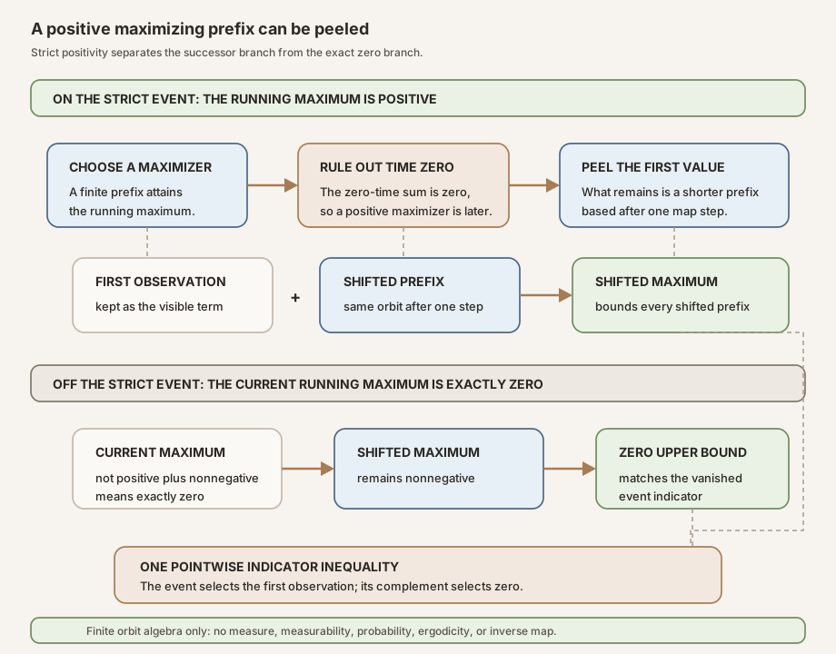
Figure: The upper lane shows the event branch. Strict positivity forces the maximizing horizon to be a successor, so the first observation can be peeled away and the remaining prefix is bounded by the shifted running maximum. The lower lane shows the complement branch: the current maximum equals zero, the shifted maximum is nonnegative, and the indicator vanishes. Together the lanes give one pointwise inequality. This is a conceptual diagram with no empirical quantities.
Peel a positive maximizing index
The proof now reaches its algebraic heart. The task is to compare the maximum at \(\omega\) with the maximum at \(T\omega\). A maximizing prefix at the original point contains one first observation plus a shorter prefix based at the shifted point.
On the event
finiteBirkhoffSumMax_le_on_finiteHopfEvent assumes
\(\omega\in E_N(g)\) and proves
The proof applies Finset.exists_mem_eq_sup’ to obtain an index \(k\) that
attains the maximum. Since the maximum is positive, the corresponding sum is
positive. The case \(k=0\) collapses to the impossible inequality
\(0\lt0\). Therefore \(k=j+1\) for some \(j\).
Mathlib’s successor identity for Birkhoff sums is
\[ S_{j+1}g(\omega)=g(\omega)+S_jg(T\omega). \]The remainder index \(j\) is no larger than \(N\), so \(S_jg(T\omega)\le M_Ng(T\omega)\). Substituting the maximizing equality finishes the event branch. The exact finite sum definition and successor identities come from pinned Mathlib (Birkhoff-sum API).
Notice what is not used. The map need not be measurable. It need not be injective or invertible. No measure exists in this theorem’s statement. The proof compares two finite lists of real numbers linked by the orbit recursion.
Off the event
Suppose \(\omega\notin E_N(g)\). The maximum is not positive, but it is always nonnegative. Antisymmetry therefore gives
\[ M_Ng(\omega)=0. \]The shifted maximum remains nonnegative, so
\[ M_Ng(\omega)-M_Ng(T\omega)=-M_Ng(T\omega)\le0. \]The indicator of \(E_N(g)\) is also zero off the event. This branch is the reason including the zero-time sum is so convenient.
One inequality carries both branches
finiteBirkhoffSumMax_sub_comp_le_indicator combines the cases:
On the event, the indicator returns \(g(\omega)\) and the peeling theorem supplies the bound. Off the event, the indicator returns zero and the nonnegative shifted maximum supplies the bound.
The theorem is pointwise for every \(\omega\). It is stronger than an almost-everywhere inequality and costs no analytic assumptions. Measurability and integrability enter only when both sides are integrated.
Integrate and cancel the shifted maximum
The private helper
integral_comp_of_measurePreserving appears next in the source. It
states that if \(T\) preserves \(\mu\) and \(g\) is integrable, then
This is not a change-of-variables theorem requiring an inverse. The proof uses
the pushforward measure. Mathlib’s integral_map identifies the
integral of \(g\circ T\) under \(\mu\) with the integral of \(g\) under
Measure.map T μ, given the relevant almost-everywhere
measurability. The field hT.map_eq rewrites that pushforward back
to \(\mu\)
(Bochner integral under a map).
The helper is private because it is proof-local infrastructure, not a new project-wide API. Mathlib already exposes general measure-preserving composition facts, including propagation of integrability (integrable composition).
The finite Hopf-style maximal ergodic lemma
integral_finiteHopfEvent_nonneg is the core public theorem:
theorem integral_finiteHopfEvent_nonneg
    (hT : MeasurePreserving T μ μ) (hg : Integrable g μ) (N : ℕ) :
    0 ≤ ∫ ω in finiteHopfEvent T g N, g ω ∂μ
Its proof has five auditable stages.
Abbreviate the finite maximal function by \(M\) and its strict event by \(E\).
Prove \(M\) integrable. Measure preservation then makes \(M\circ T\) integrable as well.
Obtain null-measurability of \(E\). This makes the indicator \(\mathbf 1_Eg\) integrable even if the raw representative of \(g\) was not ordinarily measurable.
Integrate the pointwise inequality:
\[ \int(M-M\circ T)\,d\mu\le\int\mathbf 1_Eg\,d\mu. \]Use preservation to identify the two maximal integrals. The left side is zero. Mathlib’s null-measurable indicator identity rewrites the right side as the set integral \(\int_Eg\,d\mu\) (indicator and set-integral API).
The result follows:
\[ 0\le\int_{E_N(g)}g\,d\mu. \]Why the assumptions are genuinely lean
The measure may have infinite total mass. The count-measure probe later gives
an explicit infinite-measure instance. It may also be the zero measure. No
IsFiniteMeasure, IsProbabilityMeasure, or
sigma-finiteness typeclass appears.
The map may be noninjective. A constant Boolean map preserves a Dirac measure and satisfies the theorem. Preservation is expressed by pushforward equality, which does not require an inverse.
Ergodicity is absent. The identity map is measure preserving and the theorem applies to it for every integrable observable, even when that identity system is far from ergodic.
Preservation is not cosmetic. A separate probe constructs a measurable map and integrable observable for which preservation fails and the event integral is negative. The proof’s cancellation step identifies exactly what breaks.
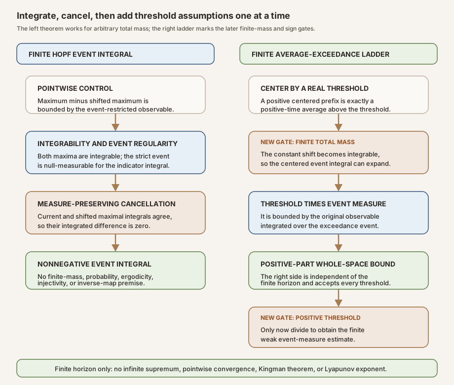
Figure: The left column follows the main finite theorem from a pointwise indicator bound through integrability and measure-preserving cancellation to a nonnegative event integral. The right column applies the result to the observable shifted by a real threshold, expands the constant set integral under finite total mass, replaces the observable by its positive part, and divides only after adding a positive-threshold premise. The figure is conceptual; the complete formulas and assumptions remain in the text.
Center first, divide last
The final eight public declarations turn the finite sum theorem into a finite average-exceedance interface. The order of operations is the key: subtract the threshold from the observable first, apply the maximal lemma, and divide by the threshold only at the very end.
Define exceedance through a centered observable
finiteBirkhoffAverageExceedanceSet is
def finiteBirkhoffAverageExceedanceSet
    (T : Ω → Ω) (g : Ω → ℝ) (N : ℕ) (a : ℝ) : Set Ω :=
  finiteHopfEvent T (fun ω ↦ g ω - a) N
At a positive horizon \(k\), finite additivity gives
\[ S_k(g-a)(\omega)=S_kg(\omega)-k a. \]Because \(k\gt0\), the centered sum is positive exactly when
\[ a\lt\frac{S_kg(\omega)}{k}=A_kg(\omega). \]The use of positive indices is essential. At time zero, division is totalized but carries no threshold information.
Membership and monotonicity
mem_finiteBirkhoffAverageExceedanceSet_iff states the precise
event meaning:
The Lean proof rewrites the centered Birkhoff sum, evaluates the constant orbit sum as \(k a\), and uses positivity of the natural index cast to justify division. It assumes no sign for \(a\).
finiteBirkhoffAverageExceedanceSet_mono says these events increase
with the cutoff \(N\), directly by monotonicity of finite Hopf events.
Measurable and null-measurable routes
measurableSet_finiteBirkhoffAverageExceedanceSet assumes ordinary
measurability of \(T\) and \(g\). Subtracting a measurable constant preserves
ordinary measurability, so the strict event is measurable.
nullMeasurableSet_finiteBirkhoffAverageExceedanceSet assumes
measure preservation, integrability of \(g\), and
[IsFiniteMeasure μ]. Finite total mass first appears because the
constant function \(\omega\mapsto a\) must be integrable. Then \(g-a\) is
integrable and the earlier null-measurable event theorem applies.
Finite total mass is weaker than probability normalization. No mass-one
identity is used. It also prevents the real-valued measure
\(\mu_{\mathbb R}(E)\) from encountering an infinite mass in the later formula.
Mathlib defines μ.real E as the real conversion of the extended
nonnegative measure; the finite-measure premise keeps this conversion in its
ordinary finite regime
(real-valued measure).
The centered integral lower bound
finiteBirkhoffAverageExceedanceSet_integral_lower_bound applies the
main theorem to \(g-a\):
Linearity and the constant set-integral formula give
\[ \int_{E_{N,a}}(g-a)\,d\mu {} =\int_{E_{N,a}}g\,d\mu-a\,\mu_{\mathbb R}(E_{N,a}). \]Rearranging yields
\[ a\,\mu_{\mathbb R}(E_{N,a}) \le\int_{E_{N,a}}g\,d\mu. \]The theorem accepts every real \(a\). For \(a=0\), the left side is zero. For negative \(a\), the inequality remains valid but should not be narrated as a useful upper bound on event size. No division has occurred.
A horizon-independent positive-part bound
finiteBirkhoffAverageExceedanceSet_posPart_bound continues with two
order comparisons. Pointwise,
The positive part is nonnegative, so its integral over a subset is no larger than its integral over the whole space. Therefore
\[ a\,\mu_{\mathbb R}(E_{N,a}) \le\int_\Omega\max(g,0)\,d\mu. \]Mathlib supplies integrability of the positive part of an integrable real function and the required set-integral monotonicity lemmas (positive parts and monotone set integrals). The right side no longer depends on \(N\). The theorem still assumes no sign for \(a\).
Positivity enters at division
measureReal_finiteBirkhoffAverageExceedanceSet_le finally assumes
\(0\lt a\) and divides the previous inequality by \(a\):
This is the finite weak maximal estimate. The positivity premise belongs exactly here because order-preserving division by a real scalar requires a positive denominator. Adding \(0\lt a\) to earlier theorems would make their interfaces unnecessarily strong; omitting it here would make the division invalid.
The estimate is finite in \(N\). It has the correct uniform right side for a later increasing-event passage, but that passage is not part of this module.
The exact premise and nonclaim ledger
The theorem family has four layers. Reading them together prevents assumptions from leaking backward and conclusions from leaking forward.
| Layer | Main declarations | Exact positive assumptions | Explicitly absent |
|---|---|---|---|
| Finite order algebra | finiteBirkhoffSumMax through finiteBirkhoffSumMax_zero | A map, a real observable, a natural horizon; an index bound where stated | Measurability, measure, integrability, preservation, finite mass, probability, ergodicity, invertibility |
| Regularity and event algebra | Measurable/integrable maximum, event regularity, membership, monotonicity, horizon identities, peeling, indicator inequality | Ordinary measurability for the measurable route; preservation plus integrability for the integrable route; no analytic premise for raw event algebra | Probability, ergodicity, injectivity, surjectivity, inverse dynamics, convergence |
| Finite Hopf integral | integral_finiteHopfEvent_nonneg | MeasurePreserving T μ μ, Integrable g μ, finite horizon | Finite total mass, probability normalization, sigma-finiteness, ergodicity, invertibility, ordinary measurability of the chosen \(g\) representative |
| Threshold and weak estimate | Average-exceedance declarations | Finite total mass, preservation, integrability; additionally \(0\lt a\) only for the final divided bound | Probability, ergodicity, infinite-horizon supremum, almost-everywhere convergence |
What the main theorem does not claim
- that \(E_N(g)\) has positive measure;
- that \(E_N(g)\) tends to a measurable infinite-horizon event;
- that the measures of the finite events converge;
- that a supremum over all \(N\) is integrable;
- that Birkhoff averages converge at any point;
- that the Birkhoff convergence event from RMT-22 is conull;
- that a pointwise Birkhoff theorem has been proved;
- that the limit, if it exists, equals a conditional expectation;
- that the transformation is ergodic or mixing;
- that an additive result automatically proves a subadditive Kingman theorem;
- that the project’s log-positive cocycle observable has a samplewise growth rate;
- that a signed Lyapunov exponent or an Oseledets splitting exists.
Why “finite Hopf-style lemma” is a descriptive name
“Finite” fixes the horizon. “Hopf-style” acknowledges the operator lineage and the pointwise maximum-minus-shift proof. “Lemma” signals that this is an analytic component of a longer pointwise development, not the final maximal ergodic theorem in infinite time. The name avoids attributing the exact Lean statement to a historical source whose hypotheses or proof differ.
The complete source-order tour
The following inventory follows the frozen 509-line module exactly. The private helper is included where it occurs, between public declarations 16 and 17.
Finite maximum declarations
finiteBirkhoffSumMaxdefines the running maximum of the Birkhoff sums at horizons zero through \(N\), using a proof-carrying nonempty finite supremum.birkhoffSum_le_finiteBirkhoffSumMaxbounds every prefix with index at most \(N\) by that maximum.finiteBirkhoffSumMax_nonneginserts the zero-horizon sum to prove pointwise nonnegativity.finiteBirkhoffSumMax_monoproves monotonicity when the horizon is enlarged.finiteBirkhoffSumMax_zerocomputes the zero-horizon maximum as zero and is tagged for simplification.measurable_finiteBirkhoffSumMaxobtains ordinary measurability from ordinary measurability of the map and observable.integrable_finiteBirkhoffSumMaxobtains integrability from measure preservation and integrability of the one-step observable, without a finite-measure assumption.
Strict event declarations
finiteHopfEventdefines the strict positivity event of the finite running maximum.measurableSet_finiteHopfEventgives the ordinary measurable-set route.nullMeasurableSet_finiteHopfEvent_of_integrablegives the null-measurable route used by the integral theorem.mem_finiteHopfEvent_iffconverts membership into existence of a positive Birkhoff sum at an index between one and \(N\).finiteHopfEvent_monoproves that the finite events increase with the horizon.finiteHopfEvent_zerocomputes the zero-horizon event as empty.mem_finiteHopfEvent_one_iffidentifies the one-horizon event with strict positivity of \(g\).
Pointwise and integrated Hopf declarations
finiteBirkhoffSumMax_le_on_finiteHopfEventchooses a positive maximizing successor index and peels its first orbit value.finiteBirkhoffSumMax_sub_comp_le_indicatorjoins the event and complement branches into the pointwise maximum-minus-shift indicator inequality.
The private helper integral_comp_of_measurePreserving proves
integral invariance under composition from integral_map and
hT.map_eq. It is not counted among the twenty-five public
declarations.
integral_finiteHopfEvent_nonnegintegrates the pointwise inequality, cancels the two maximal-function integrals, and rewrites the indicator integral as the set integral.
Average-threshold declarations
finiteBirkhoffAverageExceedanceSetdefines finite average exceedance by applying the strict event to \(g-a\).mem_finiteBirkhoffAverageExceedanceSet_iffidentifies event membership with a positive-time average exceeding the threshold.finiteBirkhoffAverageExceedanceSet_monoproves horizon monotonicity.measurableSet_finiteBirkhoffAverageExceedanceSetsupplies the ordinary measurable-set route.nullMeasurableSet_finiteBirkhoffAverageExceedanceSetsupplies the finite-measure, integrable null-measurable route.finiteBirkhoffAverageExceedanceSet_integral_lower_boundexpands the centered event integral to put threshold times real measure below the integral of \(g\) on the event, for every real threshold.finiteBirkhoffAverageExceedanceSet_posPart_boundreplaces the event integral by the whole-space integral of the positive part, still for every real threshold.measureReal_finiteBirkhoffAverageExceedanceSet_leassumes a positive threshold and divides to obtain the finite weak measure estimate.
The three final #print axioms commands inspect the core event
integral, the centered lower bound, and the divided weak estimate. They are
audit commands, not additional declarations.
Eleven probes test the theorem’s edges
The source ends with eleven anonymous examples. They compile with the module and therefore test actual elaboration, not informal intention.
Probe 1: horizon zero is empty
For arbitrary \(T\) and \(g\), the first probe reuses
finiteHopfEvent_zero. The resulting identity records that
totalization introduces no positive value at horizon zero.
Probe 2: horizon one sees exactly \(g\gt0\)
The second probe reuses mem_finiteHopfEvent_one_iff. It checks the
indexing convention: one Birkhoff step contains the observation at the current
point.
Probe 3: the zero observable never enters
For every horizon, the strict event of the identically zero observable is empty. This checks that the supremum and strict inequality do not create a spurious witness.
Probe 4: the nonnegative event is universal
The set
\[ \{\omega:0\le M_Ng(\omega)\} \]is the whole space. This probe is the executable reason not to define the Hopf event with a weak inequality.
Probe 5: identity dynamics needs no ergodicity
For the identity map, every integrable \(g\) satisfies the main nonnegative event-integral theorem under any measure. This instantiation records that the theorem has no ergodicity hypothesis.
Probe 6: the zero measure is allowed
An arbitrary measurable map, the zero observable, and the zero measure satisfy the theorem. The result is mathematically degenerate but type-correct. No nonzero-mass or probability assumption is hidden.
Probe 7: infinite counting measure is allowed
The count measure on the natural numbers is not finite. The probe constructs an integrable observable supported at zero, with value one there, and applies the theorem to identity dynamics. This instantiation records that finite total mass is not among the core finite Hopf lemma’s hypotheses.
Probe 8: a noninjective preserving map is allowed
On the Boolean type, the constant map to false is not injective
but preserves the Dirac measure at false. The theorem applies at
horizon three. This blocks any accidental invertibility narrative.
Probe 9: preservation is necessary
The next Boolean example uses the Dirac measure at true, a map
that sends every point to false, and an observable equal to minus
one at true and two at false. The map is measurable
and the observable is integrable, but the map does not preserve the Dirac
measure. At horizon two, true enters the strict event while the
set integral is negative.
This is a boundary countermodel, not a proof that preservation is the only possible sufficient hypothesis. It shows that the public conclusion fails if preservation is dropped while the displayed remaining conditions are kept.
Probe 10: the centered lower bound accepts a negative threshold
Under finite measure, the integral lower bound is instantiated at \(a=-1\). The example checks the declaration’s true quantifier: positivity is not needed before division.
Probe 11: the weak bound exposes positive division
The final probe restates the weak measure estimate with an explicit \(0\lt a\) hypothesis. Its signature places positivity at the final divided bound, where the proof uses it.
What the probes collectively rule out
| Potential accidental premise or convention | Probe evidence |
|---|---|
| Positive horizon required for the core theorem | Horizon zero compiles and gives the empty event |
| Weak event inequality is informative | The corresponding event is proved universal |
| Observable must be nonzero | Zero observable compiles and gives an empty event |
| Ergodicity required | Identity dynamics compiles |
| Nonzero or finite total mass required | Zero measure and infinite counting measure both compile |
| Injectivity or invertibility required | Constant noninjective Dirac-preserving map compiles |
| Preservation is unused decoration | A nonpreserving counterexample makes the conclusion false |
| Threshold must be positive in the centered integral theorem | The negative-threshold instance compiles |
| Division can be stated without a sign premise | The final interface explicitly requires \(0\lt a\) |
Proof engineering lessons
RMT-23 is short by the standards of the surrounding subadditive development, but it exposes several reusable Lean techniques.
Use a nonempty finite supremum when zero is a real candidate
One tempting definition is a fold with default zero. That would happen to
produce the same real value here because time zero is present, but it would
hide the structural reason. sup’ records nonemptiness explicitly
and gives the exact witness APIs needed later. The proof does not depend on a
default-order convention.
Extract a maximizing index only when needed
Most properties of the maximum use order lemmas and do not need to choose an index. The proof extracts a maximizer only for horizon monotonicity and the peeling step. This keeps finite choice local and makes the positive-index argument visible.
Separate event regularity from pointwise event algebra
The event definition, membership theorem, monotonicity, edge horizons, and pointwise inequality need no measure. Measurability appears in separate declarations. This avoids forcing analytic assumptions into reusable finite algebra.
Prefer null-measurability when that is all integration needs
An integrable function comes with almost-everywhere strong measurability, not necessarily ordinary measurability of the chosen representative. Requiring an ordinary measurable \(g\) in the main theorem would strengthen the interface without helping the proof. The null-measurable event route matches Mathlib’s indicator and set-integral APIs directly.
Cancel through pushforward equality, not an inverse
Writing an informal substitution such as “let \(y=T\omega\)” can tacitly
assume bijectivity. The Lean proof does not. It builds the equality through
Measure.map T μ and rewrites with preservation. This is both more
more general and more precise.
Keep the sign gate at the operation that consumes it
Centering by \(a\), integrating, and bounding by the positive part work for every real \(a\). Only division changes order according to the sign of \(a\). The source therefore adds \(0\lt a\) only to the final theorem. This is a model for assumption-minimal APIs elsewhere in the project.
Failure modes the source avoids
- Terminal-positive-part confusion. The running maximum is over every partial sum, not \(\max(S_N,0)\).
- Weak-event collapse. Defining the event by \(0\le M_N\) makes it universal because time zero is included.
- Zero-index peeling. A maximizing index can be peeled only after strict positivity proves it is a successor.
- Ordinary-measurability inflation. Integrability already supplies the almost-everywhere regularity needed for the main integral.
- Hidden inverse substitution. Integral cancellation comes from pushforward equality, not from solving \(T\omega=y\).
- Premature finite measure. The core theorem works on infinite measures; finite mass is introduced only for constant centering.
- Premature positive threshold. The centered inequalities accept all real thresholds; positivity is needed only for division.
- Finite-to-infinite overreach. Uniform finite estimates do not themselves prove the measurability, continuity from below, integrability, or convergence steps required by an infinite-horizon theorem.
Worked derivation without Lean syntax
Fix \(\omega\) and \(N\). There are two cases.
If \(M_Ng(\omega)\gt0\), choose \(k\le N\) with \(S_kg(\omega)=M_Ng(\omega)\). Strict positivity implies \(k=j+1\). Then
\[ \begin{aligned} M_Ng(\omega) &=S_{j+1}g(\omega)\\ &=g(\omega)+S_jg(T\omega)\\ &\le g(\omega)+M_Ng(T\omega). \end{aligned} \]Rearranging gives
\[ M_Ng(\omega)-M_Ng(T\omega)\le g(\omega). \]If \(M_Ng(\omega)\) is not positive, nonnegativity forces it to be zero. Hence
\[ M_Ng(\omega)-M_Ng(T\omega)=-M_Ng(T\omega)\le0. \]The indicator of the strict event selects the right side appropriate to each case. Integrate. Preservation gives
\[ \int M_Ng\circ T\,d\mu=\int M_Ng\,d\mu, \]so the integrated left side is zero. The indicator integral is the set integral over the strict event. That proves the core lemma.
For the threshold corollary, replace \(g\) by \(g-a\). The strict event becomes the set where some positive-time average exceeds \(a\). Then
\[ 0\le\int_{E_{N,a}}(g-a)\,d\mu {} =\int_{E_{N,a}}g\,d\mu-a\,\mu_{\mathbb R}(E_{N,a}). \]Move the constant term to the other side. Bound \(g\) by its positive part. Only if \(a\gt0\), divide by \(a\). Every public theorem corresponds to one of these logically separate moves.
Exercises with solutions
Exercise 1: distinguish two maxima
For prefix sums \(0,4,-3\), compute the running maximum through time two and the positive part of the terminal sum.
Solution. The running maximum is four. The terminal sum is minus three, so its positive part is zero. The objects differ.
Exercise 2: explain nonemptiness
Why can finiteBirkhoffSumMax use sup’ even when
\(N=0\)?
Solution. Finset.range (N + 1) contains zero for every natural
\(N\). At \(N=0\), it is the singleton containing zero.
Exercise 3: locate nonnegativity
Which candidate proves \(M_N\ge0\)?
Solution. The time-zero Birkhoff sum. It equals zero and is one of the values over which the maximum is taken.
Exercise 4: test a weak event
What is the event \(\{\omega:0\le M_Ng(\omega)\}\)?
Solution. It is the whole space, because the maximum is pointwise nonnegative.
Exercise 5: find the witness at horizon one
Why is \(E_1(g)=\{\omega:0\lt g(\omega)\}\)?
Solution. The available sums are \(S_0=0\) and \(S_1=g\). Their maximum is strictly positive exactly when \(g\) is strictly positive.
Exercise 6: peel the maximizing prefix
Suppose the maximum is attained at \(k=j+1\). What identity exposes the first observation?
Solution. \(S_{j+1}g(\omega)=g(\omega)+S_jg(T\omega)\).
Exercise 7: explain the index bound after peeling
If \(j+1\le N\), why may the proof bound \(S_jg(T\omega)\) by the shifted maximum through \(N\)?
Solution. The inequality implies \(j\le N\), so \(j\) is one of the candidate horizons in \(M_Ng(T\omega)\).
Exercise 8: solve the off-event branch
Why is the current maximum exactly zero off the strict event?
Solution. Off the event it is not positive. The time-zero candidate makes it nonnegative. A real number that is both nonpositive and nonnegative equals zero.
Exercise 9: name the cancellation mechanism
Why does preservation identify the integrals of \(M_Ng\circ T\) and \(M_Ng\)?
Solution. Integration after composition equals integration against the
pushforward measure, and MeasurePreserving identifies that
pushforward with the original measure.
Exercise 10: reject an inverse assumption
Does the preceding argument require solving for a preimage of each point?
Solution. No. Pushforward equality is enough. The map may be noninjective and nonsurjective away from the support of the preserved measure.
Exercise 11: place ordinary measurability
Why is ordinary measurability of \(g\) absent from the core integral theorem?
Solution. Integrable g μ supplies almost-everywhere strong
measurability. That regularity is enough to make the maximal function
integrable, the strict event null-measurable, and the event indicator
integrable.
Exercise 12: place finite mass
Why does finite total mass enter when the observable is centered by \(a\)?
Solution. The constant function with value \(a\) must be integrable so that \(g-a\) is integrable and its set integral can be expanded. A general constant need not be integrable on an infinite-measure space.
Exercise 13: convert centered sums to averages
For \(k\gt0\), show that \(S_k(g-a)\gt0\) is equivalent to \(A_kg\gt a\).
Solution. Expand \(S_k(g-a)=S_kg-ka\), move \(ka\) across the inequality, and divide by the positive real number \(k\).
Exercise 14: test the zero threshold
What does the centered lower bound say when \(a=0\)?
Solution. It says \(0\le\int_{E_{N,0}}g\,d\mu\), recovering the core Hopf inequality for the unshifted observable under this corollary’s stronger finite-measure premise.
Exercise 15: test a negative threshold
Why does the lower bound remain valid for \(a\lt0\), while the final weak measure estimate does not use that case?
Solution. Centering and integral rearrangement do not divide by \(a\). The final estimate divides by \(a\) while preserving order, which requires a positive denominator.
Exercise 16: find the horizon-independent quantity
Which term in the weak bound does not depend on \(N\)?
Solution. The whole-space integral of the positive part, \(\int\max(g,0)\,d\mu\).
Exercise 17: audit the infinite-measure model
Which finite-mass hypothesis is absent from the core theorem?
Solution. The counting-measure model has a nonfinite measure, an integrable nonzero observable, and measure-preserving dynamics for which the core theorem applies. The declaration’s signature has no finite-total-mass premise.
Exercise 18: audit the nonpreserving probe
What may be concluded from the Boolean counterexample with a negative event integral?
Solution. The displayed conclusion does not follow from mere measurability of the map and integrability of the observable. It does not prove that measure preservation is logically necessary among every conceivable alternative hypothesis.
Exercise 19: separate finite and infinite maxima
Does monotonicity of \(E_N\) by itself prove an infinite-horizon maximal inequality?
Solution. No. A later proof must define the union or supremum, establish its regularity, pass the finite inequalities to the limit, and justify each measure or integral convergence step.
Exercise 20: place the pointwise theorem
Does the finite weak estimate prove that Birkhoff averages converge almost everywhere?
Solution. No. A pointwise proof needs additional approximation and oscillation or density arguments. RMT-23 supplies one maximal component, not the convergence theorem.
Reproducibility and audit ledger
| Artifact | Role | Validation |
|---|---|---|
FiniteHopfMaximal.lean | Twenty-five documented public declarations, one private integral helper, eleven anonymous probes, and three axiom-print commands | Direct warning-fatal Lean check, aggregator/root build, boundary review, and axiom audit |
RandomCocycles.lean | Aggregator import for the new module | Warning-fatal aggregator and root checks |
This index.md | Declaration-complete and probe-complete proof-to-prose map | Teaching source hygiene, coverage manifest, and Hugo warnings fatal |
positive-maximizer-peeling.svg | Event/complement proof split and positive-index peeling | UTF-8 XML parse and rendered inspection |
integration-cancellation-threshold-ladder.svg | Integral cancellation and threshold assumption ladder | UTF-8 XML parse and rendered inspection |
generate-card.sh | Deterministic featured-card generator | CWD-independent –verify byte comparison and 1200x630 dimension check |
From the repository root:
source "$HOME/.elan/env"
cd formalization
lake env lean -DwarningAsError=true \
  NonlinearDynamics/Random/RandomCocycles/FiniteHopfMaximal.lean
lake build NonlinearDynamics.Random.RandomCocycles.FiniteHopfMaximal
lake env lean -DwarningAsError=true \
  NonlinearDynamics/Random/RandomCocycles.lean
lake env lean -DwarningAsError=true NonlinearDynamics/Random.lean
lake env lean -DwarningAsError=true NonlinearDynamics.lean
cd ..
python3 scripts/check_teaching_source_hygiene.py
python3 scripts/check_lean_notebook_coverage.py
make site-check
The public-surface audit should include:
import NonlinearDynamics

open MeasureTheory Set
open NonlinearDynamics.Random.RandomCocycles

#check finiteBirkhoffSumMax
#check finiteBirkhoffSumMax_nonneg
#check finiteHopfEvent
#check mem_finiteHopfEvent_iff
#check finiteBirkhoffSumMax_sub_comp_le_indicator
#check integral_finiteHopfEvent_nonneg
#check finiteBirkhoffAverageExceedanceSet
#check mem_finiteBirkhoffAverageExceedanceSet_iff
#check finiteBirkhoffAverageExceedanceSet_integral_lower_bound
#check finiteBirkhoffAverageExceedanceSet_posPart_bound
#check measureReal_finiteBirkhoffAverageExceedanceSet_le
The integrated source is 509 lines with SHA-256
3f385c36fae5d0483ea592468d4d79d197e74a4e241b63f859b0aaace03a8b58.
That hash freezes the exact Lean authority audited by this chapter. The source
contains no proof hole or custom axiom. Its three #print axioms
commands inspect the core finite Hopf theorem, the centered threshold lower
bound, and the divided weak estimate.
This article publishes as an open working note with draft: false and
retains pro_reviewed: false. Deterministic builds, declaration coverage,
source hygiene, and visual inspection do not replace human mathematical,
historical, accessibility, and editorial review.
The next ridge
The finite events \(E_{N,a}\) are increasing in \(N\), and their measure has a right-hand bound independent of \(N\) when \(a\gt0\). Their increasing-event passage is now formalized in the successor chapter, From Every Finite Horizon to One Infinite Event in Lean. That chapter defines the infinite event, proves its measurable and null-measurable presentations, identifies it with the union of the finite events, and passes the finite bound through extended and real measure continuity with the explicit sufficient finiteness premise visible.
An infinite maximal inequality would still not finish the pointwise Birkhoff theorem. A complete route needs a dense class on which convergence is already known, control of approximation errors by the maximal estimate, and a closed or otherwise stable convergence set. The precise Koopman and function-space interfaces must be audited against pinned Mathlib before choosing that slice.
The subadditive program remains further away. A pointwise additive theorem can eventually supply frequencies or averages for measurable favorable sets, but Kingman’s theorem must also connect centered subadditive processes, phase averaging, interval packing, finite maximal control, invariant limits, and the integrated Fekete rate. No one of those finite components can be renamed as a samplewise growth theorem.
For matrix cocycles, the current observable is log-positive and therefore clips contraction. Signed logarithms, zero-product behavior, negative-tail integrability, singular values, exterior powers, and invariant splittings remain separate prerequisites before Lyapunov-exponent or Oseledets language is justified.
References
The primary-source links below were checked on 2026-07-21. The exact Mathlib
authority is version 4.32.0 at commit
81a5d257c8e410db227a6665ed08f64fea08e997.
Kosaku Yosida and Shizuo Kakutani. Birkhoff’s Ergodic Theorem and the Maximal Ergodic Theorem, Proceedings of the Imperial Academy 15(6), 165–168, 1939, with the open archival scan. Page 165 gives the one-to-one measure-preserving setting, explicitly does not assume finite total measure, labels Theorem 2 new, and introduces the name “Maximal Ergodic Theorem.” Pages 166–167 contain the maximal-interval proof. The paper’s infinite-horizon average formulation is historical lineage, not the exact RMT-23 theorem or proof.
Eberhard Hopf. The General Temporally Discrete Markoff Process, Journal of Rational Mechanics and Analysis 3(1), 13–45, 1954; see also the journal record. The article is cited for the broader operator-theoretic lineage. The archive exposed article-level metadata but not a freely inspectable internal theorem page during this audit, so no theorem number or page-specific mathematical claim is assigned to it here.
Adriano M. Garsia. A Simple Proof of E. Hopf’s Maximal Ergodic Theorem, Journal of Mathematics and Mechanics 14(3), 381–382, 1965; see the journal record. Page 381 states the finite operator theorem with \(S_0=0\), the running maximum over indices zero through \(n\), the strict positive event, the nonnegative event integral, and the pointwise maximum-minus-shift inequality. It is the closest proof source for RMT-23. Its running-maximum notation is not the positive part of the terminal sum.
Michael Keane and Karl Petersen. Easy and Nearly Simultaneous Proofs of the Ergodic Theorem and Maximal Ergodic Theorem, IMS Lecture Notes–Monograph Series 48, 248–251, 2006, with arXiv:math/0608251v1, submitted 2006-08-10. Pages 248–249 use a probability space, permit a noninvertible measure-preserving transformation, form strict finite maximal-average events, and begin the passage to the infinite theorem. The final peer-reviewed version is cited as the version of record; the arXiv copy is linked for open access.
Mathlib contributors.
Finite Birkhoff sums and successor decompositions,
Mathlib 4.32.0. These lines define birkhoffSum, identify its zero
and one horizons, and provide both successor recursions. RMT-23 uses the
first-term peeling identity birkhoffSum_succ’.
Mathlib contributors. Nonempty finite-supremum induction and application, pointwise evaluation, and strict witnesses and maximizing indices, Mathlib 4.32.0. These declarations support integrability induction, event membership, and positive-maximizer peeling.
Mathlib contributors. Measurability of finite range suprema, Mathlib 4.32.0. RMT-23 combines this API with the finite Birkhoff-sum measurability theorem imported from RMT-22.
Mathlib contributors. Integrability under a measure-preserving composition, Mathlib 4.32.0. This API carries the finite maximal function through one application of the base map.
Mathlib contributors.
Bochner integrals under measurable pushforward,
Mathlib 4.32.0. The private cancellation helper combines
integral_map with MeasurePreserving.map_eq; it does not
use an inverse transformation.
Mathlib contributors. Indicators of null-measurable sets and set integrals and constant set integrals, Mathlib 4.32.0. These APIs convert the integrated indicator into the event integral and expand the centered constant term.
Mathlib contributors. Integrability of the positive part and monotonicity of restricted integrals, Mathlib 4.32.0. They justify the horizon-independent positive-part bound.
Mathlib contributors.
Definition of the real-valued measure projection,
Mathlib 4.32.0. μ.real s is the real conversion of the extended
nonnegative value μ s; RMT-23’s threshold layer assumes finite total
measure.
The exact upstream revision audited for this chapter is commit
81a5d257,
the revision pinned by formalization/lake-manifest.json.