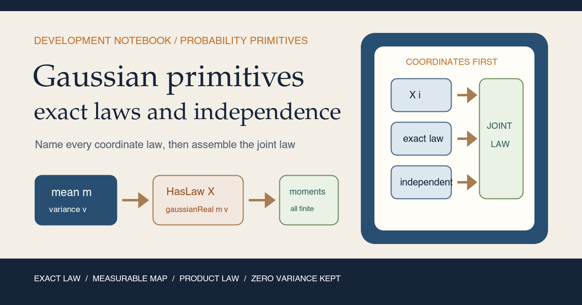
This is the code companion to
formalization/NonlinearDynamics/Random/GaussianPrimitives.lean. Every named
declaration in that file is explained below. The checked Lean source is the
authority when notation in the prose is abbreviated.
The reusable mathematical background is developed in Gaussian Laws, Independence, and Normalization. Four compact Knowledge Base entries are useful while reading: Gaussian distribution , variance , independence , and normalization convention .
Choose a route up
| Route | Begin with | Destination |
|---|---|---|
| First probability encounter | A bell curve is not yet a random variable | Separate a sample map from its law |
| Measure-theory route | Five layers | Distinguish measurable, a.e. measurable, exact law, and qualitative Gaussianity |
| Lean route | The exact scalar interface | Read every theorem and its upstream proof engine |
| Independence route | From coordinates to a vector | See why mutual independence is a joint-law statement |
| Constructor route | The canonical product sample space | Obtain a concrete family with any finite parameter schedule |
| Random-matrix route | The next ridge | Identify exactly what remains before complex entries and GUE |
Learning objectives
By the summit, a reader should be able to:
- explain why
HasRealGaussianLaw X m v Pis stronger than saying only that \(X\) is Gaussian; - distinguish
Measurable XfromAEMeasurable X P; - explain why variance is represented by
ℝ≥0rather than an unconstrained real; - derive mean, variance, integrability, and
MemLp X p Pfor every \(p\ne\infty\) from an exact law; - explain the zero-variance Gaussian as a Dirac law rather than an exception to be discarded;
- track the mean and variance through scaling and an independent sum;
- distinguish pairwise independence from
iIndepFun, the mutual independence used here; - read
Measure.pias the joint product law of a finite family; - explain why the family record stores ordinary measurability separately;
- construct a canonical finite independent Gaussian family from coordinate projections; and
- state every claim that is still absent from the random-matrix roadmap.
The ascent in one picture
flowchart TB
  A["sample map X : Omega -> Real"] --> B["ordinary measurable?"]
  A --> C["HasLaw X (gaussianReal m v) P"]
  C --> D["a.e. measurable"]
  C --> E["mean m and variance v"]
  C --> F["MemLp for p not infinity, and integrable"]
  C --> G["qualitative HasGaussianLaw"]
  C --> H["v = 0 means X = m a.e."]
  I["coordinate maps X i"] --> J["ordinary measurable + exact laws + mutual independence"]
  J --> K["IndependentRealGaussianFamily"]
  K --> L["joint law = finite product of coordinate laws"]
  K --> M["jointly Gaussian after forgetting parameters"]
  N["canonical product sample space"] --> O["coordinate evaluations"]
  O --> K
  P["complex splitting + matrix normalization"] -. future .-> Q["GUE constructor"]
  K -. primitive input .-> P
Reading the proof graph. The solid
arrows are checked in GaussianPrimitives.lean. An exact law gives
almost-everywhere measurability, but the arrow to ordinary measurability does
not exist. The family record therefore asks for ordinary measurability as
separate evidence. The dotted path is future work: no complex variable, matrix
ensemble, or GUE normalization is introduced here.
Why scalar Gaussians come before Gaussian matrices
In random-matrix physics, a matrix entry is not merely a number written in a grid. It is a random variable. A Hermitian matrix also couples entries: off-diagonal coordinates occur in conjugate pairs, while diagonal coordinates must be real. A Gaussian unitary ensemble adds another layer by specifying the joint Gaussian law and a dimension-dependent variance convention.
Those statements are easy to compress into the phrase “take Gaussian entries.” Formalization makes the hidden choices visible:
- Which measure is the law of each real coordinate?
- Is the second parameter a variance or a standard deviation?
- Are different primitive coordinates mutually independent?
- How does a deterministic scale factor transform the variance?
- What happens when the variance or scale is zero?
- What is the exact joint law of the coordinate vector?
- Which variances will later be assigned to diagonal, real off-diagonal, and imaginary off-diagonal parts?
The current module answers the first six questions while deliberately leaving the seventh open. That order prevents a later matrix definition from assuming a normalization convention merely through convenient notation.
The historical physics motivation is spectral statistics. Wigner introduced random matrices as models for complicated spectra, and Dyson organized ensembles by symmetry class. Those primary papers motivate the broader program; they do not determine this file’s Lean interface or prove a modern GUE normalization (Wigner 1955; Dyson 1962).
Lineage, local contribution, and nonclaims
The Gaussian density, product measures, independence, and closure of independent Gaussians under addition are classical. Mathlib 4.32.0 already contains the underlying measures and theorems. This module does not reprove the analytic normalization integral or characteristic-function identities.
Its local contribution is an interface shaped for later random matrices:
- a short exact-law predicate with explicit mean and variance;
- named consequences that keep those parameters available;
- a zero-variance API that includes degenerate Gaussians explicitly;
- scaling and independent-addition lemmas with exact parameter arithmetic;
- a family record that stores ordinary measurability, exact coordinate laws, and mutual independence as three separate obligations;
- coordinatewise deterministic scaling of that whole record;
- finite joint-law and joint-Gaussian conclusions; and
- a canonical product sample space whose coordinate projections realize any finite parameter schedule.
Not claimed
- No complex Gaussian random variable is defined.
- No choice is made for how a complex variance is split between real and imaginary parts.
- No random matrix, Wigner matrix, GOE, or GUE law is constructed.
- No diagonal or off-diagonal matrix variance is selected.
- No density formula is rederived in this project module.
- No covariance matrix for a dependent Gaussian vector is introduced.
- No eigenvalue, spectral measure, unitary-invariance, trace-moment, or asymptotic theorem follows from this file.
- No ordinary measurability is inferred from
HasLaw; where it is needed, the record asks for it explicitly.
Base camp: a bell curve is not yet a random variable
For positive variance \(v\gt 0\), the familiar real Gaussian density with mean \(m\) and variance \(v\) is
\[ x\longmapsto \frac{1}{\sqrt{2\pi v}} \exp\!\left(-\frac{(x-m)^2}{2v}\right). \]Mathlib packages the corresponding measure as gaussianReal m v. Its second
parameter has type ℝ≥0, Lean’s nonnegative real numbers. The type rules out
negative variance before any theorem begins.
The boundary value \(v=0\) needs special care. Substituting zero into the density formula would divide by zero. Mathlib instead defines
\[ \operatorname{gaussianReal}(m,0)=\delta_m, \]the Dirac probability measure concentrated at \(m\). This choice gives a closed parameter space: scaling a Gaussian by zero still has a Gaussian law, and zero-variance coordinates can coexist with nondegenerate coordinates in a product.
A sample map and a law have different jobs
Let \((\Omega,\mathcal F,P)\) be a measure space. A function
\[ X:\Omega\to\mathbb R \]assigns a real value to every outcome. It is the sample map. The law records how \(P\)-mass is transported through \(X\):
\[ \mathcal L_P(X)=P\circ X^{-1}. \]Mathlib writes this pushforward as P.map X. Its HasLaw X μ P structure
contains two facts:
Xis almost-everywhere measurable underP;P.map X = μ.
The project’s exact Gaussian predicate specializes \(\mu\) to
gaussianReal m v.
Five layers that must not be collapsed
| Layer | Lean form | What it says | What it does not say |
|---|---|---|---|
| Sample map | X : Ω → ℝ | Every outcome is assigned a real | No event compatibility or probability law yet |
| Ordinary measurability | Measurable X | Every measurable target event has a measurable preimage | No particular distribution |
| A.e. measurability | AEMeasurable X P | X agrees \(P\)-a.e. with a measurable map | The original representative need not be ordinarily measurable |
| Exact Gaussian law | HasRealGaussianLaw X m v P | The pushforward is exactly gaussianReal m v | It does not supply ordinary measurability |
| Qualitative Gaussian law | HasGaussianLaw X P | The pushforward is Gaussian in Mathlib’s general sense | The chosen \(m\) and \(v\) are no longer parameters of the proposition |
The distinction between the last two layers is central. A later matrix constructor needs exact variances, not merely a certificate that every coordinate belongs to some Gaussian class. The distinction between ordinary and almost-everywhere measurability is equally important. Matrix assembly is often defined pointwise, so the family interface retains ordinary measurable coordinate maps.
Camp one: the exact scalar interface
The first declaration is only one line:
def HasRealGaussianLaw (X : Ω → ℝ) (m : ℝ) (v : ℝ≥0) (P : Measure Ω) : Prop :=
  HasLaw X (gaussianReal m v) P
HasRealGaussianLaw
NonlinearDynamics.Random.HasRealGaussianLaw is a transparent definition,
not a new probability theory. Unfolding it gives Mathlib’s HasLaw. This
thin wrapper gives the project a stable vocabulary and fixes the parameter
order used by every later constructor.
The type of \(v\) does real work. A term of type ℝ≥0 contains a real value
and a proof that the value is nonnegative. The module never asks downstream
users to carry a separate hypothesis 0 ≤ v.
HasRealGaussianLaw.aemeasurable
theorem aemeasurable (hX : HasRealGaussianLaw X m v P) : AEMeasurable X P :=
  ProbabilityTheory.HasLaw.aemeasurable hX
This theorem is a named projection from the underlying HasLaw evidence. The
proof architecture is direct delegation. It intentionally returns
AEMeasurable X P, not Measurable X.
That restraint matters because two functions equal outside a null set have the same pushforward law under the almost-everywhere machinery, even if one chosen representative behaves badly on the null set.
HasRealGaussianLaw.isProbabilityMeasure
theorem isProbabilityMeasure (hX : HasRealGaussianLaw X m v P) :
    IsProbabilityMeasure P :=
  ProbabilityTheory.HasLaw.isProbabilityMeasure hX
Every gaussianReal m v is a probability measure, including \(v=0\).
Mathlib’s HasLaw.isProbabilityMeasure transports that normalization back to
the source. Thus the existence of an exact Gaussian variable rules out a
source measure with total mass different from one.
This is a property of the whole source measure, not only of the image. The
almost-everywhere measurability stored in HasLaw is what prevents the
degenerate fallback behavior of Measure.map from manufacturing a misleading
zero law.
HasRealGaussianLaw.mean_eq
theorem mean_eq (hX : HasRealGaussianLaw X m v P) :
    ∫ ω, X ω ∂P = m := by
  rw [ProbabilityTheory.HasLaw.integral_eq hX, integral_id_gaussianReal]
The proof has two rewrites:
HasLaw.integral_eqchanges the integral of \(X\) under \(P\) into the integral of the identity function under the target law.integral_id_gaussianRealevaluates that canonical Gaussian integral as \(m\).
In symbols,
\[ \int_\Omega X(\omega)\,dP(\omega) {} = \int_{\mathbb R}x\,d\operatorname{gaussianReal}(m,v)(x) {} = m. \]The first equality is transport by law. The second is the Gaussian moment calculation already proved in Mathlib.
HasRealGaussianLaw.variance_eq
theorem variance_eq (hX : HasRealGaussianLaw X m v P) :
    Var[X; P] = (v : ℝ) := by
  simpa using ProbabilityTheory.HasLaw.variance_eq hX
HasLaw.variance_eq transports variance to the identity map on the target
measure. Mathlib then simplifies the variance of gaussianReal m v to \(v\).
The displayed coercion (v : ℝ) forgets the nonnegativity proof so both sides
live in the real numbers.
The mean does not appear in the final expression because variance is centered:
\[ \operatorname{Var}_P(X) {} = \int_\Omega\!\left(X-\mathbb E_PX\right)^2\,dP {} = v. \]HasRealGaussianLaw.hasGaussianLaw
theorem hasGaussianLaw (hX : HasRealGaussianLaw X m v P) :
    HasGaussianLaw X P :=
  ProbabilityTheory.HasLaw.hasGaussianLaw hX
This is a forgetful step. Mathlib records gaussianReal m v as a Gaussian
measure, so an exact HasLaw proof yields the broader HasGaussianLaw
predicate.
The implication points one way in this interface:
\[ \text{exact parameters} \Longrightarrow \text{qualitative Gaussianity}. \]The theorem does not recover parameters from arbitrary qualitative evidence. That asymmetry is healthy. Later matrix code should keep exact parameters until it intentionally forgets them.
HasRealGaussianLaw.memLp
theorem memLp (hX : HasRealGaussianLaw X m v P)
    (p : ℝ≥0∞) (hp : p ≠ ∞) : MemLp X p P :=
  (hasGaussianLaw hX).memLp hp
The theorem covers every exponent p ≠ ∞, including Mathlib’s p = 0 case.
The exponent lives in ℝ≥0∞, the extended nonnegative reals, so the side
condition precisely excludes only the infinite endpoint.
The exponent-zero case is degenerate: MemLp X 0 P records
almost-everywhere strong measurability here, not a numerical \(L^0\) norm or
a finite zeroth-moment claim. Ordinary positive moments begin with positive
natural exponents.
For each positive natural \(k\), choose \(p=k\). Then
\[ \int_\Omega |X(\omega)|^k\,dP(\omega)\lt\infty. \]This is the integrability foundation later polynomial matrix entries and trace moments will need. It does not yet prove any matrix-valued observable is integrable.
The proof first forgets the explicit parameters with hasGaussianLaw, then
uses Mathlib’s general Gaussian memLp theorem. That upstream theorem rests on
the analytic tail control developed for Gaussian measures; this project
reuses it rather than rebuilding the analysis.
HasRealGaussianLaw.integrable
theorem integrable (hX : HasRealGaussianLaw X m v P) : Integrable X P :=
  (hasGaussianLaw hX).integrable
Integrability is the \(L^1\) case exposed under its standard name. It licenses
the ordinary expectation interpretation of mean_eq. The proof again travels
through qualitative Gaussianity and Mathlib’s general theorem.
Camp two: the mountain includes zero variance
A reusable API should not force every later theorem to split into \(v\gt 0\) and \(v=0\) unless a density argument truly requires it. Two declarations make the degenerate boundary explicit.
HasRealGaussianLaw.ae_eq_const_of_variance_zero
theorem ae_eq_const_of_variance_zero
    (hX : HasRealGaussianLaw X m 0 P) :
    X =ᵐ[P] fun _ ↦ m := by
  apply ProbabilityTheory.HasLaw.ae_eq_of_dirac
  simpa only [HasRealGaussianLaw, gaussianReal_zero_var] using hX
The proof rewrites gaussianReal m 0 as Measure.dirac m, then applies the
general theorem that a variable with Dirac law equals the atom almost
everywhere.
The conclusion is almost-everywhere equality. The law cannot control values on a \(P\)-null set, so pointwise equality would overclaim.
HasRealGaussianLaw.zero_variance_iff
theorem zero_variance_iff [IsProbabilityMeasure P] :
    HasRealGaussianLaw X m 0 P ↔ X =ᵐ[P] fun _ ↦ m := by
  rw [HasRealGaussianLaw, gaussianReal_zero_var, hasLaw_dirac_iff]
The reverse direction needs the source to be a probability measure. If \(X=m\) almost everywhere under an arbitrary finite measure, its pushforward is the source mass times \(\delta_m\), not necessarily \(\delta_m\). The typeclass assumption supplies total mass one.
This equivalence is stronger than the preceding one because it supports construction: under a probability measure, an almost-surely constant map is a valid zero-variance Gaussian primitive.
Edge cases covered here
| Case | Exact result |
|---|---|
| \(v=0\) | The law is \(\delta_m\), and \(X=m\) \(P\)-a.e. |
| \(m=0,v=0\) | The variable is zero \(P\)-a.e. |
| A null-set modification of a constant | It has the same zero-variance law, but need not be pointwise constant |
| Source mass not known to be one | The forward Dirac implication holds from HasLaw; the reverse equivalence is not available |
Camp three: exact laws survive basic operations
The first downstream users will rescale Gaussian coordinates and add independent pieces. The module gives both operations exact parameter formulas.
HasRealGaussianLaw.const_mul
theorem const_mul (hX : HasRealGaussianLaw X m v P) (c : ℝ) :
    HasRealGaussianLaw (fun ω ↦ c * X ω) (c * m)
      (⟨c ^ 2, sq_nonneg c⟩ * v) P :=
  gaussianReal_const_mul hX c
The mathematical rule is
\[ X\sim\mathcal N(m,v) \quad\Longrightarrow\quad cX\sim\mathcal N(cm,c^2v). \]The term ⟨c ^ 2, sq_nonneg c⟩ constructs a nonnegative real from \(c^2\)
and its proof of nonnegativity. The theorem delegates to Mathlib’s exact
pushforward law for scalar multiplication.
Three boundary checks are built into the same statement:
- If \(c\lt 0\), the mean changes sign as appropriate while the variance uses \(c^2\).
- If \(c=0\), the output law is the zero-variance Dirac law at zero.
- If \(v=0\), scaling a deterministic Gaussian remains deterministic.
No positivity assumption on \(c\) or \(v\) is hidden.
HasRealGaussianLaw.add_of_indep
theorem add_of_indep
    (hX : HasRealGaussianLaw X mX vX P)
    (hY : HasRealGaussianLaw Y mY vY P)
    (hXY : IndepFun X Y P) :
    HasRealGaussianLaw (fun ω ↦ X ω + Y ω)
      (mX + mY) (vX + vY) P := by
  simpa only [HasRealGaussianLaw, gaussianReal_conv_gaussianReal] using
    hXY.hasLaw_fun_add hX hY
Independence is the bridge from separate laws to the law of the sum.
IndepFun.hasLaw_fun_add says that the sum law is the convolution of the two
coordinate laws. gaussianReal_conv_gaussianReal evaluates the convolution:
The simpa unfolds the local exact-law wrapper and rewrites Gaussian
convolution. The proof is short because Mathlib already owns the hard
characteristic-function argument.
Two worked scalar laws
Suppose \(X\sim\mathcal N(0,1)\). Applying const_mul with \(c=2\) gives
If \(X\) and \(Y\) are independent with
\(X,Y\sim\mathcal N(0,1)\), add_of_indep gives
Combining the two theorems yields the normalized sum
\[ \frac{X+Y}{\sqrt 2}\sim\mathcal N(0,1). \]This last display is a paper derivation from the two checked closure rules. No standalone Lean theorem with the square-root simplification is named in this file.
High camp: from coordinates to a vector
A matrix needs many primitive variables at once. Writing an exact law beside each coordinate is not enough. The family also needs ordinary measurability for pointwise assembly and mutual independence for a product joint law.
IndependentRealGaussianFamily
structure IndependentRealGaussianFamily
    (X : ι → Ω → ℝ) (m : ι → ℝ)
    (v : ι → ℝ≥0) (P : Measure Ω) : Prop where
  measurable : ∀ i, Measurable (X i)
  hasLaw : ∀ i, HasRealGaussianLaw (X i) (m i) (v i) P
  independent : iIndepFun X P
The four inputs are:
X, an indexed family of real sample maps;m, the mean schedule;v, the nonnegative variance schedule; andP, the common source measure.
The three fields answer different questions:
| Field | Obligation | Why later matrix code needs it |
|---|---|---|
measurable | Every X i is ordinarily measurable | Finite coordinate assembly and deterministic transforms can use pointwise measurable APIs |
hasLaw | Coordinate i has exactly gaussianReal (m i) (v i) | Diagonal and off-diagonal scales remain visible |
independent | The whole indexed family satisfies iIndepFun | The joint law factors as a product |
The index type \(\iota\) is unrestricted at the structure level. Finiteness appears only when the module forms a finite product measure or invokes finite-dimensional joint Gaussianity.
iIndepFun expresses mutual independence of the family, not only pairwise
independence. For more than two variables, pairwise independence does not in
general determine the joint product law. The stronger field is exactly what
jointHasLaw will consume.
IndependentRealGaussianFamily.aemeasurable
theorem aemeasurable
    (hX : IndependentRealGaussianFamily X m v P) (i : ι) :
    AEMeasurable (X i) P :=
  (hX.measurable i).aemeasurable
This theorem weakens the record’s ordinary measurable field to the almost-everywhere form. It does not need the coordinate law. That proof choice documents which field is authoritative for sample-map regularity.
IndependentRealGaussianFamily.isProbabilityMeasure
theorem isProbabilityMeasure
    (hX : IndependentRealGaussianFamily X m v P) :
    IsProbabilityMeasure P :=
  hX.independent.isProbabilityMeasure
Mathlib’s mutual-independence predicate carries probability normalization. Using that field also handles an empty index type cleanly, where there is no coordinate law to select.
For a nonempty family, any hX.hasLaw i would also imply source
normalization. The chosen proof avoids an unnecessary nonemptiness
assumption.
Coordinate mean and variance
theorem mean_eq
    (hX : IndependentRealGaussianFamily X m v P) (i : ι) :
    ∫ ω, X i ω ∂P = m i :=
  (hX.hasLaw i).mean_eq

theorem variance_eq
    (hX : IndependentRealGaussianFamily X m v P) (i : ι) :
    Var[X i; P] = (v i : ℝ) :=
  (hX.hasLaw i).variance_eq
IndependentRealGaussianFamily.mean_eq and
IndependentRealGaussianFamily.variance_eq are fieldwise forwarding
theorems. Each selects the exact coordinate law and applies the corresponding
scalar theorem. Mutual independence is not needed for a marginal mean or
variance.
IndependentRealGaussianFamily.scale
theorem scale
    (hX : IndependentRealGaussianFamily X m v P) (c : ι → ℝ) :
    IndependentRealGaussianFamily
      (fun i ω ↦ c i * X i ω)
      (fun i ↦ c i * m i)
      (fun i ↦ ⟨(c i) ^ 2, sq_nonneg (c i)⟩ * v i) P := by
  refine ⟨fun i ↦ (hX.measurable i).const_mul (c i),
    fun i ↦ (hX.hasLaw i).const_mul (c i), ?_⟩
  simpa only [Function.comp_def] using
    hX.independent.comp
      (fun i x ↦ c i * x)
      (fun i ↦ measurable_const_mul (c i))
This proof rebuilds all three record fields:
- ordinary measurability is preserved by multiplication by a constant;
- each exact law is transformed by
HasRealGaussianLaw.const_mul; and - mutual independence is preserved by applying a measurable deterministic function to each coordinate separately.
The last point is subtle. A shared transform that mixes coordinates could
create dependence. Coordinate \(i\) here uses only \(X_i\), through the
measurable map \(x\mapsto c_i x\), so iIndepFun.comp applies.
Zero scale factors are allowed. A scaled coordinate may become deterministic while remaining independent of the others. This is useful for sparse constructions and for dimensions where a coefficient vanishes.
The product-law gate
The next two theorems add [Fintype ι]. The family record itself remains
general, but the current project needs a finite coordinate vector for a finite
matrix.
IndependentRealGaussianFamily.jointHasLaw
theorem jointHasLaw
    (hX : IndependentRealGaussianFamily X m v P) :
    HasLaw (fun ω i ↦ X i ω)
      (Measure.pi fun i ↦ gaussianReal (m i) (v i)) P :=
  hX.independent.hasLaw_pi hX.hasLaw
The joint sample map sends one outcome to the full coordinate vector:
\[ \omega\longmapsto\bigl(i\mapsto X_i(\omega)\bigr). \]Its law is the finite product
\[ \bigotimes_{i\in\iota}\mathcal N(m_i,v_i). \]This theorem is the formal payoff of mutual independence. The coordinate laws
identify every marginal; iIndepFun says those marginals factor jointly;
Mathlib’s iIndepFun.hasLaw_pi combines the two pieces.
The result is exact. It names the full measure on \(\iota\to\mathbb R\), not only a list of marginal statements.
IndependentRealGaussianFamily.jointHasGaussianLaw
theorem jointHasGaussianLaw
    (hX : IndependentRealGaussianFamily X m v P) :
    HasGaussianLaw (fun ω i ↦ X i ω) P :=
  hX.independent.hasGaussianLaw
    fun i ↦ (hX.hasLaw i).hasGaussianLaw
Independent Gaussian coordinates form a jointly Gaussian finite vector. Mathlib proves this general fact through characteristic functions. The local proof supplies:
- mutual independence from the record; and
- qualitative Gaussianity of each coordinate by forgetting its exact parameters.
jointHasLaw and jointHasGaussianLaw are related but not redundant:
| Theorem | Retains \(m_i,v_i\)? | Best use |
|---|---|---|
jointHasLaw | Yes, in the explicit product measure | Exact coordinate calculations and constructors |
jointHasGaussianLaw | No | General linear-image and Gaussian-vector theory |
Summit camp: the canonical product sample space
So far, every theorem begins with random variables that already exist. The final declarations provide a canonical realization.
gaussianProductMeasure
noncomputable def gaussianProductMeasure [Fintype ι]
    (m : ι → ℝ) (v : ι → ℝ≥0) : Measure (ι → ℝ) :=
  Measure.pi fun i ↦ gaussianReal (m i) (v i)
The sample space is the coordinate space itself, \(\iota\to\mathbb R\). A sample \(x\) is already a complete vector. Its \(i\)th random variable is evaluation, \(x\mapsto x_i\).
The definition is noncomputable because it constructs an abstract
measure-theoretic object, not a sampler or pseudorandom-number generator.
Nothing here generates floating-point Gaussian samples.
instIsProbabilityMeasureGaussianProduct
instance instIsProbabilityMeasureGaussianProduct [Fintype ι]
    (m : ι → ℝ) (v : ι → ℝ≥0) :
    IsProbabilityMeasure (gaussianProductMeasure m v) := by
  unfold gaussianProductMeasure
  infer_instance
Each coordinate Gaussian is a probability measure. Mathlib’s product-measure instance turns their finite product into a probability measure. After unfolding the project definition, typeclass inference closes the proof.
This works for an empty finite index type. The empty product is the Dirac measure at the unique empty tuple and has total mass one. That is a convention for this scalar product space only; it does not decide whether a future matrix ensemble accepts or rejects dimension zero.
gaussianProductMeasure_hasLaw_eval
theorem gaussianProductMeasure_hasLaw_eval [Fintype ι]
    (m : ι → ℝ) (v : ι → ℝ≥0) (i : ι) :
    HasRealGaussianLaw (fun x : ι → ℝ ↦ x i)
      (m i) (v i) (gaussianProductMeasure m v) := by
  exact
    (measurePreserving_eval
      (fun i ↦ gaussianReal (m i) (v i)) i).hasLaw
Evaluation at coordinate \(i\) is measure-preserving from the product measure
to its \(i\)th factor. A measure-preserving map has the corresponding
HasLaw, so the coordinate projection has exactly the requested Gaussian
law.
The theorem is unavailable for an empty index only because no term i : ι
can be supplied. The product measure itself and the family constructor below
remain valid.
gaussianProductMeasure_iIndepFun
theorem gaussianProductMeasure_iIndepFun [Fintype ι]
    (m : ι → ℝ) (v : ι → ℝ≥0) :
    iIndepFun (fun i (x : ι → ℝ) ↦ x i)
      (gaussianProductMeasure m v) := by
  exact iIndepFun_pi
    (μ := fun i ↦ gaussianReal (m i) (v i))
    (X := fun _ ↦ id) fun _ ↦ aemeasurable_id
Coordinate projections under a product measure are mutually independent.
Mathlib’s iIndepFun_pi states this construction principle. The local proof
chooses the identity map in every factor and supplies its
almost-everywhere measurability.
Notice the direction of reasoning:
- define the product measure;
- prove coordinate laws by evaluation;
- prove coordinate independence from the product structure.
Earlier, jointHasLaw went in the other direction: given coordinate laws and
independence on an arbitrary source, identify its joint law as the product.
Together the two directions show that the abstract interface has a canonical
model.
gaussianProductMeasure_independentFamily
theorem gaussianProductMeasure_independentFamily [Fintype ι]
    (m : ι → ℝ) (v : ι → ℝ≥0) :
    IndependentRealGaussianFamily
      (fun i (x : ι → ℝ) ↦ x i) m v
      (gaussianProductMeasure m v) :=
  ⟨fun i ↦ measurable_pi_apply i,
    gaussianProductMeasure_hasLaw_eval m v,
    gaussianProductMeasure_iIndepFun m v⟩
The final constructor fills the family record in its field order:
measurable_pi_apply iproves ordinary measurability of evaluation;gaussianProductMeasure_hasLaw_evalsupplies every exact coordinate law;gaussianProductMeasure_iIndepFunsupplies mutual independence.
This is the theorem a later finite random-matrix constructor can call when it needs a concrete independent family with a declared variance schedule.
The entire Lean file as a declaration map
The table uses fully qualified names where short names repeat across namespaces.
| Declaration | Role | Proof engine |
|---|---|---|
HasRealGaussianLaw | Exact scalar Gaussian law with \(m,v,P\) visible | Definition by HasLaw X (gaussianReal m v) P |
HasRealGaussianLaw.aemeasurable | A.e. measurability | Underlying HasLaw field |
HasRealGaussianLaw.isProbabilityMeasure | Source mass is one | HasLaw.isProbabilityMeasure |
HasRealGaussianLaw.mean_eq | Expectation equals \(m\) | Transport integral, then integral_id_gaussianReal |
HasRealGaussianLaw.variance_eq | Variance equals \(v\) | HasLaw.variance_eq and Gaussian simplification |
HasRealGaussianLaw.hasGaussianLaw | Forget exact parameters | HasLaw.hasGaussianLaw |
HasRealGaussianLaw.memLp | MemLp X p P for every p ≠ ∞, including p = 0 | General Gaussian memLp |
HasRealGaussianLaw.integrable | Finite first absolute moment | General Gaussian integrable |
HasRealGaussianLaw.ae_eq_const_of_variance_zero | Zero variance implies a.e. constancy | Rewrite Gaussian to Dirac |
HasRealGaussianLaw.zero_variance_iff | Dirac-law equivalence under probability source | hasLaw_dirac_iff |
HasRealGaussianLaw.const_mul | Exact deterministic scaling | gaussianReal_const_mul |
HasRealGaussianLaw.add_of_indep | Exact independent sum | Addition law, convolution, Gaussian convolution |
IndependentRealGaussianFamily | Measurable exact independent coordinate bundle | Three-field structure |
IndependentRealGaussianFamily.aemeasurable | Coordinate a.e. measurability | Weaken ordinary measurable field |
IndependentRealGaussianFamily.isProbabilityMeasure | Family source mass is one | Independence predicate |
IndependentRealGaussianFamily.mean_eq | Coordinate expectation | Scalar mean_eq |
IndependentRealGaussianFamily.variance_eq | Coordinate variance | Scalar variance_eq |
IndependentRealGaussianFamily.scale | Coordinatewise scaling of the bundle | Measurable scaling, exact scalar law, iIndepFun.comp |
IndependentRealGaussianFamily.jointHasLaw | Exact finite product joint law | iIndepFun.hasLaw_pi |
IndependentRealGaussianFamily.jointHasGaussianLaw | Qualitative joint Gaussianity | Independent Gaussians are jointly Gaussian |
gaussianProductMeasure | Canonical product-space measure | Measure.pi |
instIsProbabilityMeasureGaussianProduct | Product is probabilistic | Typeclass inference |
gaussianProductMeasure_hasLaw_eval | Exact marginal of evaluation | measurePreserving_eval |
gaussianProductMeasure_iIndepFun | Mutual independence of evaluations | iIndepFun_pi |
gaussianProductMeasure_independentFamily | Canonical full bundle | Constructor from measurability, laws, independence |
Proof architecture: why the file is short
The local module is an adapter layer over a deep upstream library. Its proofs follow four recurring moves.
1. Unfold an exact law
HasRealGaussianLaw exposes HasLaw when a Mathlib theorem requires it.
Because the wrapper is definitionally transparent, most adaptations need only
simpa or a direct theorem application.
2. Transport a quantity through equality in law
Mean and variance are calculated on the canonical target measure, not by integrating the original sample map from scratch. This is the central payoff of an exact law:
\[ P\mathbin{\mathrm{map}}X=\mu \quad\Longrightarrow\quad \text{distributional functionals of }X {} = \text{those of the identity under }\mu. \]3. Preserve structure under coordinatewise maps
Scaling proves the three family obligations separately. The independence proof uses measurable coordinatewise composition, never a heuristic that “deterministic operations preserve independence” without stating which operations see which coordinates.
4. Move between marginals and joint laws
On an arbitrary source, exact marginals plus mutual independence produce the product joint law. On the canonical product source, coordinate projections recover those marginals and independence. This two-way bridge makes the interface usable both abstractly and constructively.
Exact commands: compile, cover, and preview
From the repository root on macOS or Linux:
source "$HOME/.elan/env"
cd formalization
lake env lean -DwarningAsError=true NonlinearDynamics/Random/GaussianPrimitives.lean
lake build
cd ..
The first command loads elan into the shell. The direct lean command
checks this module with warnings promoted to errors. lake build then checks
the complete import graph.
Starting from the repository root, build the complete formalization and check the public teaching content:
cd formalization
lake build

cd ..
make content-hygiene
make site-check
lake build checks the complete project import graph. The final two commands
inspect the public teaching content and render the site.
Regenerate the conceptual card from any working directory:
site/content/development-notebook/2026/07/\
gaussian-primitives-exact-laws-and-independence/generate-card.sh
The generator resolves its output relative to its own file, strips time-dependent PNG metadata, and checks the final dimensions. The card is a conceptual teaching figure and contains no empirical data.
Edge-case register
| Situation | What the checked API does | Common wrong inference |
|---|---|---|
| \(v=0\) | Uses a Dirac law and proves a.e. constancy | “Gaussian” must have a density |
\(c=0\) in const_mul or scale | Produces a zero-variance coordinate | Scaling theorem needs c ≠ 0 |
| \(c\lt 0\) | Mean changes by \(c\), variance by \(c^2\) | Variance changes sign |
p = ∞ | memLp theorem intentionally does not apply | Gaussian variables are essentially bounded |
A null-set modification of X | Exact law can remain unchanged | Equality in law gives pointwise equality |
| Empty finite index type | Product measure and family exist; the evaluation theorem cannot be instantiated because no i : ι exists | Empty product has mass zero |
| Arbitrary index type in the record | Record is allowed | Current finite joint-law theorem is automatically infinite-dimensional |
Exact marginal laws without iIndepFun | No product joint law follows | Gaussian marginals determine dependence |
| Pairwise independence only | Not the field stored here | Pairwise independence always implies mutual independence |
Qualitative HasGaussianLaw | Gaussian class is known | Named mean and variance remain syntactic parameters |
Exact HasLaw | A.e. measurability is known | Ordinary Measurable follows automatically |
| Independent sum | Variances add | The same formula holds without independence or covariance control |
Failure modes this interface is designed to prevent
Calling a parameter-free fact an exact law
HasGaussianLaw X P is valuable for general Gaussian-vector theorems, but a
GUE constructor needs exact variance coefficients. Use
HasRealGaussianLaw X m v P until the parameters are no longer needed.
Treating almost-everywhere measurability as ordinary measurability
The scalar exact law exposes only AEMeasurable. The family record’s
measurable field is not redundant documentation. It is stronger data used
by pointwise constructions and preserved explicitly by scale.
Declaring independent entries in prose only
The joint-law theorem consumes iIndepFun. If independence is missing from
the Lean assumptions, a product law cannot be claimed in the notebook,
either.
Hiding a standard-deviation convention
Mathlib’s gaussianReal m v uses variance. Writing an informal scale
\(\sigma\) and passing it directly as \(v\) would be off by a square. The
normalization ledger for a future matrix ensemble must state both the scale
coefficient and the resulting variance.
Dropping degenerate coordinates
Zero variance and zero scale are valid. Excluding them would complicate empty, sparse, or boundary constructions and would make scaling less compositional.
Jumping from scalar moments to matrix moments
memLp controls each scalar Gaussian. A trace power is a polynomial in many
coordinates, so later files still need a finite-product integrability
argument. This module does not prove
\(\mathbb E[\operatorname{tr}(H^k)]\) exists or compute it.
A normalization rehearsal without choosing GUE
Let \(I\) be a finite set of primitive-coordinate labels. Choose functions
\[ m:I\to\mathbb R, \qquad v:I\to\mathbb R_{\ge 0}. \]gaussianProductMeasure m v creates the product law, and
gaussianProductMeasure_independentFamily m v supplies its coordinate
projections as an independent family.
Now choose deterministic scales \(c:I\to\mathbb R\). The theorem scale
produces new parameters
This is exactly the algebra a matrix normalization will need. What the module refuses to do is decide which labels represent diagonal coordinates, which represent real or imaginary off-diagonal parts, or how \(c_i\) depends on the matrix dimension \(n\). Those are ensemble conventions, not consequences of Gaussian probability.
Exercises
The next ridge: from real coordinates to matrices
The next layer is an explicit complex Gaussian primitive. It must state whether a complex variable is defined from independent real and imaginary parts, and how a target complex second moment is split between them.
After that, a finite Hermitian Gaussian matrix constructor needs:
- an index type for independent primitive coordinates;
- a map from those coordinates to diagonal and upper-triangular entries;
- conjugate reflection into the lower triangle;
- ordinary measurability of the assembled matrix;
- a proof of Hermiticity;
- exact diagonal and off-diagonal laws;
- a normalization ledger fixing every variance and dimension factor;
- a stated policy for the zero-dimensional matrix; and
- only then, a theorem identifying and analyzing the resulting matrix law.
Unitary invariance is not automatic from the word “Gaussian.” It will require
a proof that the selected Hermitian Gaussian law is preserved by unitary
conjugation. The existing RandomMatrices.Laws module provides the language
for that statement; GaussianPrimitives provides scalar raw material.
Summit register
The module has reached a precise summit. One real Gaussian coordinate carries
an exact law with named mean and variance. That law yields a.e. measurability,
source normalization, exact first two moments, MemLp X p P for every
p ≠ ∞ (including Mathlib’s p = 0 case), integrability, exact
zero-variance behavior, deterministic scaling, and independent addition.
At family scale, ordinary measurability, exact marginal laws, and mutual independence remain distinct fields. Coordinatewise scaling preserves all three. For finite families, those fields produce both an exact product joint law and qualitative joint Gaussianity. The canonical product sample space shows that the interface is inhabited for every finite parameter schedule.
The file does not yet contain a Gaussian matrix. That is not incompleteness hidden behind a name. It is the formal boundary that keeps complex variance splitting and GUE normalization available for explicit review.
References
The technical references below were opened and checked against official Mathlib documentation and pinned source on 2026-07-20. Historical physics references link to their original journal DOI records.
Mathlib contributors.
Mathlib 4.32.0 release,
commit
81a5d257c8e410db227a6665ed08f64fea08e997.
This is the exact library revision pinned by the repository.
Mathlib contributors.
Law of a random variable,
with
pinned source.
This is the primary API source for HasLaw, its a.e.-measurability field,
transport of integrals and variance, Dirac-law equivalences, and finite
product-law theorems.
Mathlib contributors.
Real Gaussian distributions,
with
pinned source.
This is the primary API source for gaussianReal, its zero-variance Dirac
case, probability instance, mean, variance, finite moments, scaling, and
Gaussian convolution.
Mathlib contributors.
Gaussian random variables,
with
pinned source.
This is the primary API source for qualitative HasGaussianLaw, Gaussian
MemLp, and integrability.
Mathlib contributors. Gaussian independence source, with generated documentation. This is the primary API source for the theorem that finite independent Gaussian coordinates are jointly Gaussian.
Mathlib contributors.
Finite product measures,
with
pinned source.
This is the primary API source for Measure.pi, coordinate evaluation, and
independence under a product measure.
Mathlib contributors.
Independence of families,
with
pinned source.
This is the primary API source for IndepFun, iIndepFun, and preservation
of mutual independence by measurable coordinatewise maps.
Eugene P. Wigner. Characteristic Vectors of Bordered Matrices With Infinite Dimensions, Annals of Mathematics 62(3), 548-564, 1955. This original article is cited only for historical context on random-matrix models of complex spectra.
Freeman J. Dyson. Statistical Theory of the Energy Levels of Complex Systems. I, Journal of Mathematical Physics 3, 140-156, 1962. This original article is cited for the historical symmetry-class motivation, not as support for a GUE theorem in the current module.