This is the proof-to-prose companion for
formalization/NonlinearDynamics/Random/RandomMatrices/GaussianUnitaryEnsembleMoments.lean.
Every named public declaration in that stable source is mapped below.
The immediate predecessor, From Coordinates to Symmetry, identifies the coordinate-built law with a scaled intrinsic Gaussian and proves unitary invariance. The observable itself was introduced earlier in Trace-Power Observables. The probability law and its normalization ledger come from A Finite GUE Law in Lean. The parallel textbook chapter is First Exact Finite Gaussian Unitary Ensemble Trace Moments, and the compact reusable definition is finite matrix trace moment .
Reusable definitions are indexed under trace power , matrix trace , gaussian-unitary-ensemble , normalization-convention , pushforward measure , and probability law .
Choose a route up
| Route | Begin | Destination |
|---|---|---|
| First encounter | The result in one picture | See the two proof paths and why integrability comes first |
| Probability route | Why measurability is not enough | Understand complex Bochner expectation under a matrix law |
| First-moment route | First trace: only the diagonal survives | Derive the centered trace identity |
| Geometry route | Second trace: Hermitian energy | Turn the second trace into squared Frobenius norm |
| Gaussian route | One square per normalized real coordinate | Compute the exact second moment |
| Boundary route | Dimension zero is a theorem case | Audit the empty matrix without dividing by zero |
| Lean route | The complete declaration map | Inspect all four public declarations and their proof engines |
| Integrity route | Strict nonclaims | Separate exact finite moments from spectral and asymptotic claims |
Learning objectives
By the summit, a reader should be able to:
- distinguish a measurable complex observable from an integrable one;
- explain why Mathlib’s total Bochner integral makes a separate integrability theorem scientifically important;
- read
RandomMatrix.tracePower id kas an observable on the ambient matrix probability space itself; - transport integrability and integrals through a measurable pushforward;
- derive \(\operatorname{Tr}(H)=\sum_i H_{ii}\);
- use centered diagonal Gaussian laws to compute the first trace integral;
- derive \(\operatorname{Tr}(H^2)=\|H\|_F^2\) for Hermitian \(H\);
- connect the Frobenius norm to RMT-08’s normalized real coordinates;
- justify integrability of coordinate squares from a finite Gaussian second-moment bound;
- compute the second trace integral as a finite sum of coordinate variances;
- audit the cardinality \(|I_n|=n^2\) through the checked finite equivalence rather than an informal dimension slogan;
- explain why mutual independence is not used in either expectation calculation once the exact product law is available;
- handle
n = 0without an undefined1 / 0; and - separate these finite trace identities from eigenvalue and semicircle-law results.
The result in one picture
flowchart LR
  L["GUE.matrixLaw n"] --> O1["tracePower id 1"]
  L --> O2["tracePower id 2"]
  O1 --> D["finite sum of centered diagonal coordinates"]
  D --> Z["complex integral equals zero"]
  O2 --> F["Hermitian Frobenius norm squared"]
  F --> R["sum of squares over the normalized real index"]
  R --> N["n squared coordinates at varianceScale n"]
  N --> E["complex integral equals n"]
  I["integrability"] --> O1
  I --> O2
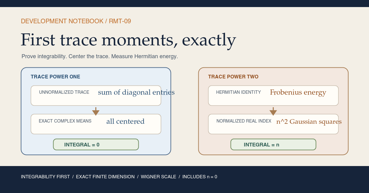
Figure. The first moment is a diagonal centering calculation. The second is an energy calculation in the normalized real Hermitian coordinates. Both paths establish Bochner integrability before evaluating a complex integral, and both include the empty zero-dimensional matrix.
The diagram has no eigenvalue node. That omission is deliberate. A matrix trace can be defined and integrated entrywise before the project chooses a measurable ordering of eigenvalues. The moment method eventually connects traces to spectral measures, as standard random-matrix references explain (Guionnet, 2022), but RMT-09 needs only finite matrix algebra and Gaussian integration.
Base camp: what exactly is being integrated?
Fix a natural dimension \(n\). The ambient sample space for this milestone is
\[ \mathcal M_n=\operatorname{Matrix}(\operatorname{Fin}(n), \operatorname{Fin}(n),\mathbb C). \]It already carries the entrywise measurable structure developed in RMT-00. The measure
\[ \mu_n=\operatorname{GUE.matrixLaw}(n) \]is a probability measure on this ambient space. It gives the measurable Hermitian locus mass one, but the observable is still a total function on all ambient matrices.
For an exponent \(k\), the project defines
\[ T_k(H)=\operatorname{Tr}(H^k). \]The Lean spelling is RandomMatrix.tracePower id k. Here id is not a
decorative argument. A RandomMatrix is a function from outcomes to matrices.
When the outcomes are matrices and the governing measure is already the
matrix law, the identity function is the canonical matrix-valued random
variable. Thus the theorem integrates the observable directly against
GUE.matrixLaw n rather than introducing a second sample space.
The codomain is \(\mathbb C\), even though trace powers are real on Hermitian matrices. This choice preserves the general observable interface. RMT-09’s equalities are therefore complex Bochner integral identities:
\[ \int_{\mathcal M_n} T_1(H)\,d\mu_n(H)=0, \qquad \int_{\mathcal M_n} T_2(H)\,d\mu_n(H)=n. \]The right side of the second identity is Lean’s complex coercion (n : ℂ).
Why measurability is not enough
RMT-01 already proved that every tracePower of a measurable finite matrix
map is measurable. Measurability permits inverse images and integration
machinery to be formed. It does not say that the integral of the norm is
finite.
For a complex-valued function \(f\), Bochner integrability combines two obligations:
- \(f\) is almost everywhere strongly measurable; and
- \(\int \|f\|\,d\mu\) is finite.
Finite-dimensional Borel measurability handles the first obligation here.
Gaussian moment bounds handle the second. The separation matters because
Mathlib defines MeasureTheory.integral as a total function and assigns a
default value outside the integrable case. The official Bochner integration
documentation states this behavior explicitly
(Mathlib Bochner integral). A bare equality involving
an unproved integral could therefore have the right-looking right side for the
wrong reason.
RMT-09 prevents that ambiguity by exporting two theorems per exponent:
| Exponent | Finiteness theorem | Evaluation theorem |
|---|---|---|
| one | GUE.integrable_tracePower_one | GUE.integral_tracePower_one |
| two | GUE.integrable_tracePower_two | GUE.integral_tracePower_two |
The ordering is part of the proof design. Each evaluation consumes an integrable finite-sum representation, not merely the fact that an integral term can be written.
Pushforward integration is the bridge to coordinates
The ambient law was not postulated by a density. It was built as a measurable pushforward of independent Gaussian coordinates. If \(A\) denotes the coordinate assembly map and \(\nu_n\) the coordinate measure, then
\[ \mu_n=A_*\nu_n. \]For a suitably measurable and integrable observable \(f\), the map theorem gives
\[ \int f(H)\,d(A_*\nu_n)(H) =\int f(A(x))\,d\nu_n(x). \]The integrability interface has the matching equivalence between a function under the mapped measure and its composition under the source measure. This is the law-level form of substitution used by the second-moment proof. The first-moment proof stays on the ambient law and consumes the exact diagonal marginal theorem directly. Both routes avoid a Lebesgue density or Jacobian.
First trace: only the diagonal survives
For every square matrix,
\[ \operatorname{Tr}(H)=\sum_{i\in\operatorname{Fin}(n)}H_{ii}. \]The GUE assembly places the real diagonal coordinate \(d_i\) directly at \(H_{ii}\). It does not double it and does not add an imaginary part. Thus, pointwise,
\[ T_1(A(d,u))=\sum_i \operatorname{ofReal}(d_i). \]The earlier theorem GUE.matrixLaw_diagonal_hasLaw states directly on the
ambient matrix law that every \(H_{ii}\) has an exact centered Cartesian
complex Gaussian law with real variance \(v_n\) and imaginary variance zero:
The project wrapper for Cartesian complex Gaussian laws exposes both integrability and the exact complex mean. Finite sums of integrable functions are integrable. Therefore the trace is integrable without reopening the coordinate pushforward.
Linearity of the Bochner integral then gives
\[ \begin{aligned} \int T_1(H)\,d\mu_n(H) &=\sum_i \int H_{ii}\,d\mu_n(H)\\ &=\sum_i 0\\ &=0. \end{aligned} \]No off-diagonal coordinate appears in the trace. No independence theorem is needed: expectation of a finite sum uses the individual integrals, whether or not the summands are independent. The exact diagonal marginal theorem already packages the coordinate construction into the ambient GUE law.
Why the result is complex zero
The exported observable and diagonal marginal theorem are both complex-valued.
The diagonal law records real variance \(v_n\) and zero imaginary variance,
but its mean field is already the complex number zero. The proof can therefore
apply .integrable and .mean_eq to each ambient diagonal entry and use
integral_finsetSum directly. No real/imaginary decomposition is needed.
Second trace: Hermitian energy
The second trace initially looks like a matrix-product observable:
\[ T_2(H)=\operatorname{Tr}(H^2) =\sum_i\sum_j H_{ij}H_{ji}. \]Hermiticity supplies \(H_{ji}=\overline{H_{ij}}\), so
\[ \operatorname{Tr}(H^2) =\sum_{i,j}H_{ij}\overline{H_{ij}} =\sum_{i,j}|H_{ij}|^2 =\|H\|_F^2. \]This identity does three jobs at once:
- it replaces a nonlinear matrix product with a norm square;
- it makes the result visibly real and nonnegative; and
- it connects directly to RMT-08’s Frobenius linear isometry.
The order of the conjugated factors is harmless in \(\mathbb C\), but Lean still needs the entrywise Hermitian equality and scalar simplification to reach the exact Frobenius expression. RMT-07’s trace-pairing theorem provides the geometric version, while the moment module specializes it to the square observable used under the integral.
One square per normalized real coordinate
RMT-08 constructs a real Euclidean index
\[ I_n=\operatorname{Fin}(n)\sqcup(T_n\sqcup T_n), \]where \(T_n\) is the strict upper triangle. Its three sectors store diagonal, normalized upper-real, and normalized upper-imaginary coordinates. A point \(x:I_n\to\mathbb R\) assembles as
\[ d_i=x_i, \qquad u_{ij}=\frac{x_{ij}^{\mathrm{re}}+ \mathrm i x_{ij}^{\mathrm{im}}}{\sqrt{2}}. \]The factor \(1/\sqrt{2}\) is exactly what makes normalized assembly a Frobenius isometry. Consequently,
\[ \operatorname{Tr}(A(x)^2) =\|A(x)\|_F^2 =\|x\|_2^2 =\sum_{a\in I_n}x_a^2. \]This is why the second trace proof does not expand diagonal and upper-triangle terms separately. The factor-two bookkeeping was already encapsulated by the isometry. A single real sum now accounts for all matrix entries with the correct multiplicity.
Integrability of a coordinate square
Every normalized coordinate has law gaussianReal 0 (varianceScale n).
Mathlib proves that a real Gaussian identity function belongs to every finite
\(L^p\) space. Taking the finite exponent two yields integrability of its
square. The module then uses finite-sum closure to prove
integrable under the common product measure. Pushforward transport and the
pointwise trace/Frobenius identity give
GUE.integrable_tracePower_two on the ambient law.
This route is stronger than arguing that every matrix entry has a finite second moment and hoping matrix multiplication preserves integrability. It names the exact scalar majorants and uses a finite number of terms.
The exact integral of one square
For a centered real random variable \(X\), variance is the second moment:
\[ \operatorname{Var}(X) =\mathbb E[(X-\mathbb E X)^2] =\mathbb E[X^2]. \]Each normalized coordinate has mean zero and variance \(v_n\), so
\[ \int x_a^2\,d\nu_n(x)=v_n. \]Finite-sum integration gives
\[ \int\operatorname{Tr}(H^2)\,d\mu_n(H) =|I_n|v_n. \]RMT-08 did not merely assert that \(I_n\) has the right dimension. It built
hermitianRealIndexEquivMatrixIndex n, an equivalence from \(I_n\) to all
matrix pairs Fin n × Fin n. Finite cardinality transport therefore yields
inside the checked proof architecture.
For a positive dimension, the approved Wigner scale is \(v_n=1/n\). Hence
\[ |I_n|v_n=n^2\frac1n=n. \]The real result is finally embedded into \(\mathbb C\), matching the codomain
of tracePower and producing (n : ℂ).
An entrywise normalization audit
The normalized-coordinate proof is the clean formal route. An independent paper audit recovers the same answer from the original GUE ledger for positive \(n\):
- the \(n\) real diagonal entries each contribute variance \(1/n\), totaling one;
- each strict-upper complex entry has real and imaginary variances \(1/(2n)\), so its expected squared modulus is \(1/n\);
- Hermiticity places that modulus once above and once below the diagonal, so each unordered off-diagonal pair contributes \(2/n\); and
- the \(n(n-1)/2\) such pairs contribute \(n-1\).
The total is \(1+(n-1)=n\). This audit explains the physics convention, but the Lean proof benefits from having the factor two absorbed once and for all by the normalized isometry.
Why independence disappears from the final arithmetic
The full GUE construction requires an exact joint product law. That law rules out hidden correlations and makes the matrix measure the intended ensemble. The final first two expectations, however, are sums of one-coordinate functions:
\[ \sum_i d_i, \qquad \sum_a x_a^2. \]Linearity of expectation uses only the marginal integral of each summand. Cross terms would require covariance or independence if the observable were, for example, the square of the trace:
\[ \left(\sum_i d_i\right)^2. \]That is a different observable from \(\operatorname{Tr}(H^2)\). Conflating the two is a common error. RMT-09’s geometric rewrite ensures the second trace contains one square for each orthonormal coordinate, not cross products among all coordinates.
This distinction is useful beyond GUE. A quadratic norm of an isotropic vector depends on the coordinate second moments. A general quadratic form or a higher trace power begins to expose correlations and combinatorics that this module does not yet formalize.
Dimension zero is a theorem case
At n = 0, the matrix carrier has one value: the empty zero matrix. The
normalized real index is also empty. The project defines
GUE.varianceScale 0 = 0, so the common Gaussian family is the unique empty
family with a Dirac law.
Every formula now reduces directly:
\[ \operatorname{Tr}(0)=0, \qquad \operatorname{Tr}(0^2)=0, \qquad |I_0|v_0=0. \]Both observables are constant zero and therefore integrable. Their complex
integrals are zero, and the second theorem’s right side (0 : ℂ) is also
zero.
The scalar simplification \(n^2(1/n)=n\) is valid only in the positive branch.
The Lean proof splits zero from successor dimension before performing field
arithmetic. It never evaluates an informal \(1/0\). This is not cosmetic edge
case work: it keeps GUE.matrixLaw and every exported theorem total on all
natural dimensions.
The complete declaration map
The stable module exports exactly four public theorems. Definitions of the observables, GUE law, normalized assembly, variance scale, and real Gaussian interfaces live in earlier modules and are reused rather than duplicated.
| Public declaration | Exact checked content | Main proof mechanism |
|---|---|---|
GUE.integrable_tracePower_one | RandomMatrix.tracePower id 1 is complex Bochner integrable under GUE.matrixLaw n | Unfold trace one as a finite ambient diagonal sum and apply integrability of the exact Cartesian complex diagonal marginals |
GUE.integral_tracePower_one | The complex integral of RandomMatrix.tracePower id 1 under GUE.matrixLaw n is zero | integral_finsetSum and the exact zero means from matrixLaw_diagonal_hasLaw |
GUE.integrable_tracePower_two | RandomMatrix.tracePower id 2 is complex Bochner integrable under GUE.matrixLaw n | Rewrite the trace square as Frobenius norm squared, transfer through normalized assembly, and sum integrable Gaussian coordinate squares |
GUE.integral_tracePower_two | The complex integral of RandomMatrix.tracePower id 2 under GUE.matrixLaw n is (n : ℂ) | Integrate one variance per normalized real coordinate, transport cardinality through the matrix-index equivalence, and split zero from successor dimension |
The private scaffold that keeps the public API small
The source names its internal seams but does not export them. This makes the four-theorem interface easy to consume without hiding how the calculation is factored.
| Private helper | Role inside the checked proof |
|---|---|
trace_sq_hermitianToMatrix | Converts trace power two of an intrinsic Hermitian point into its squared norm using the Frobenius trace pairing |
centeredGaussian_integrable_sq | Derives integrability of a scalar square from exact Gaussian MemLp at exponent two |
centeredGaussian_integral_sq | Turns zero mean plus exact variance into the integral of a square |
normalizedRealMatrixSample | Composes the normalized real decoder with Hermitian matrix assembly |
measurable_normalizedRealMatrixSample | Supplies ordinary measurability for that composite sample map |
matrixLaw_eq_map_normalizedRealMatrixSample | Rewrites the ambient GUE law as the image of the common-variance real product |
normalizedRealMatrixSample_eq | Identifies the composite sample with intrinsic normalized assembly followed by ambient inclusion |
tracePower_two_normalizedRealMatrixSample | Rewrites trace power two pointwise as a finite sum of real coordinate squares |
integrable_sum_sq_normalizedRealCoordinates | Proves the finite coordinate-square sum integrable under the product law |
integral_sum_sq_normalizedRealCoordinates | Evaluates that real sum as cardinality times varianceScale n |
card_hermitianRealIndex | Computes the normalized real index cardinality as n * n through the checked equivalence |
card_mul_varianceScale | Splits zero from successor dimension and simplifies the final Wigner-scale arithmetic |
Checked proof order
The source follows the mathematical dependency order:
- unfold trace power one and matrix trace as an ambient finite diagonal sum;
- prove its integrability from the exact diagonal complex Gaussian marginals;
- evaluate the first integral from their centered complex means;
- rewrite the ambient law as the pushforward of the common-variance real product through normalized real assembly;
- establish the pointwise Hermitian trace-two/Frobenius identity using
inner_frobenius_eq_traceand Hermiticity; - rewrite normalized assembly through the Frobenius isometry and
EuclideanSpace.real_norm_sq_eq; - prove integrability of every real coordinate square from Gaussian
MemLpand then of the finite sum; - evaluate each square with
variance_of_integral_eq_zeroand the exact variance theorem; - reindex the finite count through
hermitianRealIndexEquivMatrixIndex; and - complete the normalization arithmetic in separate zero and successor branches.
This order keeps matrix algebra, measure transport, Gaussian scalar moments, and natural-number arithmetic from appearing in one giant goal.
Mathlib interfaces used by the proof
The proof is project-specific, but its engines are standard Mathlib interfaces.
integrable_map_measure
This theorem relates integrability against a mapped measure to integrability of a composition against the source measure, under the necessary measurable map and strong-measurability hypotheses. It moves the ambient trace-two question back to the explicit normalized real coordinate probability space.
integral_map
Once measurability is visible, this theorem evaluates a Bochner integral under
Measure.map as the integral of the composed function. It is the exact
pushforward substitution rule used to expose coordinate sums.
Finite-sum integrability and integration
The index types are finite, so integrable_finsetSum and
integral_finsetSum reduce a matrix observable to scalar obligations. No
Tonelli theorem or infinite-series convergence argument is needed.
Exact Gaussian mean, variance, and finite moments
The ambient first-moment proof consumes .integrable and .mean_eq from the
exact Cartesian complex diagonal law. The second-moment helpers use
HasRealGaussianLaw.memLp, HasRealGaussianLaw.mean_eq, and
HasRealGaussianLaw.variance_eq, which wrap Mathlib’s exact gaussianReal
theorems. The finite exponent two plus MemLp.integrable_sq justifies each
coordinate square. The official Gaussian source documents both the
zero-variance Dirac branch and finite-moment API
(Mathlib real Gaussian).
Continuous linear maps commute with integration
The second-moment source integral is real-valued, while tracePower is
complex-valued. Mathlib’s integral_complex_ofReal moves the canonical real
embedding through that integral. This prevents an ad hoc real/imaginary
decomposition and makes the final complex coercion explicit.
Finite equivalences transport sums and cardinalities
hermitianRealIndexEquivMatrixIndex carries the semantic Hermitian index to
all matrix positions. The proof uses the finite-equivalence API to replace a
sum of one constant variance over \(I_n\) with the corresponding count of
matrix pairs. No unproved formula for the strict-upper cardinality is inserted
into the moment theorem. The Euclidean norm-square expansion comes from the
official finite \(\ell^2\) API
(Mathlib finite Euclidean spaces).
Implementation seams and failure modes
A law equality is not a sample equality
GUE.matrixLaw n is a measure. The coordinate constructor is a map whose
pushforward equals that measure. Rewriting the law does not produce a
pointwise inverse sample. The proof should use Measure.map, integral_map,
and map congruence rather than assuming the ambient matrix has definitional
coordinate fields.
Complex integrability does not follow from reality almost everywhere
Knowing that a trace has zero imaginary part says nothing about the size of its real part. The proof still needs a finite first absolute moment for trace one and a finite second scalar moment for trace two.
Tr(H^2) is not (Tr H)^2
The former becomes the Frobenius norm squared for Hermitian \(H\). The latter contains cross terms among diagonal entries. Substituting one for the other would change both the proof and the probabilistic value.
The off-diagonal factor two belongs to geometry
Each strict-upper complex coordinate appears twice in the full matrix norm. If displayed real and imaginary parts are treated as orthonormal without the \(\sqrt{2}\) normalization, the expected second trace is wrong. RMT-08’s isometry is the audited interface that prevents this mistake.
A variance theorem needs centering before it becomes a second moment
Variance is the integral of \((X-\mathbb E X)^2\), not automatically of
\(X^2\). The normalized GUE coordinates have exact mean zero, and that fact
must be used before replacing the square integral by varianceScale n.
Product independence is not a license to multiply expectations
Neither proof multiplies random variables from different coordinates. Trying to force an independence theorem into a finite-sum calculation adds a false dependency and obscures linearity of expectation.
The zero-dimensional scale is total, not an informal reciprocal
varianceScale is defined separately at zero. Field simplification with
1 / n belongs only in the successor case. Performing it before the case
split can create an invalid cancellation goal.
A computed integral without an integrability theorem is insufficient
Because Mathlib’s Bochner integral is total, evaluation must not be presented as proof that the expectation exists. The public API intentionally retains both integrability theorems.
Physics meaning, kept at the checked scale
A finite Hermitian matrix is the algebraic form of a finite-dimensional quantum Hamiltonian. Its trace is the sum of energy levels and its second trace is the sum of squared energy levels once a spectral theorem and enumeration are supplied. RMT-09 does not yet formalize that eigenvalue bridge, so these sentences are classical interpretation rather than Lean theorem statements.
The first identity says that the ensemble has no net trace bias. Centering is visible at the most elementary invariant observable: the expected total energy is zero.
The second identity calibrates the energy scale. Under the project’s unnormalized trace convention,
\[ \mathbb E\operatorname{Tr}(H^2)=n. \]Equivalently, the normalized trace has expectation one for positive dimension:
\[ \mathbb E\left[\frac1n\operatorname{Tr}(H^2)\right]=1. \]This is consistent with the Wigner choice that keeps typical spectral values at order one as dimension grows. Guionnet’s ICM survey records the same GUE entry variances and explains how normalized trace powers become moments of the empirical spectral measure (Guionnet, 2022). Consistency is not a limit theorem: RMT-09 proves the exact finite identity only.
The result is also basis-free in meaning. RMT-08 proves the law is invariant under unitary conjugation, and trace powers themselves are conjugation invariant. Yet the RMT-09 computation deliberately returns to coordinates, where Gaussian moments are easiest to evaluate. Symmetry explains why the answer is intrinsic; coordinates make the finite integral checkable.
Strict nonclaims
The four theorems are exact and finite, but their scope is narrow.
- No density of the ambient or intrinsic GUE law is derived.
- No Jacobian or change-of-variables theorem is used.
- No eigenvalue function is defined or proved measurable.
- No equality between trace powers and moments of an empirical spectral measure is formalized.
- No variance, concentration, tail bound, or distribution of either trace observable is computed.
- No third or higher trace moment is evaluated.
- No Wick formula, pairing enumeration, Catalan number, or genus expansion is formalized.
- No resolvent or Stieltjes transform is introduced.
- No semicircle law, almost-sure convergence, or universality statement is proved.
- No statement about an individual physical Hamiltonian follows from an ensemble expectation.
The checked summit is exactly this: two measurable complex trace observables are now known to be integrable under the finite GUE law, and their first expectations are evaluated without spectral or asymptotic machinery.
Run the checked source
From the repository root on macOS or Linux, load elan and run the stable module through the pinned Lake environment:
source "$HOME/.elan/env"
cd formalization
lake env lean -DwarningAsError=true \
  NonlinearDynamics/Random/RandomMatrices/GaussianUnitaryEnsembleMoments.lean
The direct command checks the complete RMT-09 module with warnings promoted to errors under the pinned Mathlib 4.32.0 release. Starting from the repository root, build the full Lean library and check the public teaching content with:
cd formalization
lake build

cd ..
make content-hygiene
make site-check
This complete Lean snippet inspects the entire public interface:
import NonlinearDynamics.Random.RandomMatrices.GaussianUnitaryEnsembleMoments

open Matrix MeasureTheory ProbabilityTheory
open scoped Matrix NNReal ENNReal

open NonlinearDynamics.Random

#check GUE.integrable_tracePower_one
#check GUE.integral_tracePower_one
#check GUE.integrable_tracePower_two
#check GUE.integral_tracePower_two
Save the snippet inside formalization and run lake env lean on that file.
All four names are checked declarations; the snippet contains no omitted terms
or noncompiling ellipses.
A compact proof ledger
| Obligation | Trace one | Trace two |
|---|---|---|
| Ambient observable | tracePower id 1 | tracePower id 2 |
| Pointwise rewrite | Sum of diagonal coordinates | Squared Frobenius norm |
| Coordinate rewrite | Finite sum of centered reals | Finite sum of normalized real squares |
| Finiteness source | Gaussian first integrability | Gaussian finite second moment |
| Scalar integral | Mean zero | Variance varianceScale n after centering |
| Finite count | Fin n diagonal terms | HermitianRealIndex n, equivalent to Fin n × Fin n |
| Final arithmetic | Sum of zeros | n^2 * varianceScale n = n |
| Zero-dimensional behavior | Empty sum | Empty sum and zero scale |
| Independence used in final sum? | No | No |
This table is a reading aid, not a second theorem surface. The exact source and the declaration map above remain authoritative.
Exercises with solutions
Exercise 1: identify the sample map
Why does the theorem use tracePower id 1 rather than a separately named
random matrix?
Solution. The measure GUE.matrixLaw n already lives on the ambient matrix
space. Treating a matrix as the outcome and applying id gives the canonical
matrix-valued random variable under its own law. tracePower id 1 is therefore
the trace observable directly on that probability space.
Exercise 2: separate measurability and integrability
Give an example of the logical gap between the two notions.
Solution. A measurable real function may have an infinite integral of its absolute value under a probability measure with sufficiently heavy tails. Measurability licenses the integral construction, while integrability asserts finite norm integral. Gaussian coordinates have all finite moments, but that extra theorem must be invoked.
Exercise 3: compute the first trace
Let every diagonal coordinate satisfy \(\mathbb E d_i=0\). Which dependence assumption is needed to show \(\mathbb E\sum_i d_i=0\)?
Solution. None. A finite sum of integrable random variables may be integrated term by term. Independence matters for joint laws and products, not for linearity of expectation.
Exercise 4: distinguish two quadratic observables
Expand \(\operatorname{Tr}(H^2)\) and \((\operatorname{Tr}H)^2\).
Solution. The first is \(\sum_{i,j}H_{ij}H_{ji}\), which becomes \(\sum_{i,j}|H_{ij}|^2\) for Hermitian \(H\). The second is \(\sum_{i,j}H_{ii}H_{jj}\), which contains cross terms among diagonal coordinates. They are different functions.
Exercise 5: recover the factor two
If a strict-upper entry is \(u=x+\mathrm i y\), what is its contribution to the full Frobenius norm?
Solution. Hermiticity places \(u\) above and \(\overline u\) below the diagonal. Their squared moduli sum to \(2|u|^2=2x^2+2y^2\). The orthonormal real coordinates are therefore \(\sqrt2 x\) and \(\sqrt2 y\).
Exercise 6: compute the second trace two ways
For positive \(n\), use the entrywise variance ledger to recover the value \(n\).
Solution. Diagonal terms contribute \(n(1/n)=1\). There are \(n(n-1)/2\) upper pairs. Each complex entry has expected squared modulus \(1/n\), and it appears twice in the full norm, so the off-diagonal total is \([n(n-1)/2](2/n)=n-1\). Adding gives \(n\).
Exercise 7: audit dimension zero
Why should the proof split zero from successor dimension before simplifying the variance scale?
Solution. The informal positive-dimensional expression is \(1/n\), whose cancellation laws require nonzero \(n\). The project instead defines the scale to be zero at dimension zero. In that branch the coordinate index is empty, so both trace integrals are empty sums and no reciprocal is evaluated.
Exercise 8: locate the next combinatorial difficulty
Why will \(\mathbb E\operatorname{Tr}(H^4)\) require more machinery than the second trace?
Solution. Expanding the fourth power produces products of four entries along closed index walks. Their expectations depend on how coordinate indices pair and on independence or Gaussian Wick identities. The norm-square reduction that made the second trace diagonal in normalized coordinates no longer removes all cross terms.
The next ridge
The first two trace moments certify that the finite GUE normalization is internally coherent and that the observable/integrability layer is usable. They also mark the boundary of what can be computed without new infrastructure.
Ordered Hermitian Spectra in Lean now packages the decreasing eigenvalue vector with multiplicity, its first two trace identities, counting and zero-aware empirical measures, and the exact ambient/intrinsic GUE pushforward bridge under an explicit coordinatewise eigenvalue-measurability hypothesis. The next analytic slice must prove that hypothesis through a reusable perturbation or continuity theorem. Only then should the project identify normalized random trace powers with spectral moments unconditionally. Higher GUE trace moments require a separate combinatorial or Gaussian moment layer. Asymptotic semicircle claims require yet another limit layer and remain outside this finite module.
References
The external links below were opened and checked on 2026-07-21. The pinned local Mathlib 4.32.0 source remains the API authority for the Lean proof.
Alice Guionnet. “Rare Events in Random Matrix Theory”, Proceedings of the International Congress of Mathematicians 2022, volume 2, pages 1008–1052. DOI 10.4171/ICM2022/174. Section 1.1.1 records the centered GUE entry variances used by this project, and equation (1.7) explains the classical link between normalized trace powers and empirical spectral moments. This note uses the source for mathematical and physics context, not as a substitute for the checked finite integral proofs.
Mathlib contributors.
Mathlib 4.32.0 release,
2026. This is the exact dependency release selected by
formalization/lakefile.toml.
Mathlib contributors.
Bochner integration,
Mathlib 4 documentation. This page defines the Banach-valued integral,
documents its total behavior, and exposes integral_map, finite-sum
linearity, and the integrability interfaces used to move between coordinate
and matrix laws.
Mathlib contributors.
Real Gaussian distributions,
Mathlib 4 documentation. This page defines gaussianReal, including the
zero-variance Dirac case, and proves its exact mean, variance, and finite
moments.
Mathlib contributors.
Finite Euclidean spaces and inner products,
Mathlib 4 documentation. This page supplies the EuclideanSpace carrier and
EuclideanSpace.real_norm_sq_eq, which turns the normalized real coordinate
norm square into a finite sum of scalar squares.