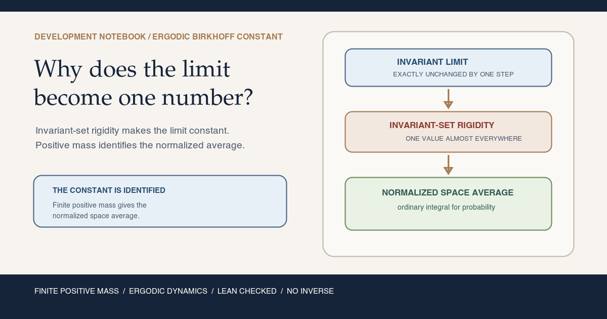
Milestone status. The RMT-28 module compiles with warnings treated as
errors. Its six public declarations report only propext,
Classical.choice, and Quot.sound, the same standard Mathlib footprint as
the preceding development. The chapter and its figures are published as an
open working note while human review remains pending.
For the reusable concepts, see the glossary entries on ergodicity , normalized space averages , conditional expectation , and the invariant sigma algebra . For a longer mathematical treatment with worked models, see Ergodic Birkhoff Limits and Normalized Space Averages.
The missing step after RMT-27
The pointwise ergodic theorem is often compressed into the slogan “time average equals space average.” That slogan hides two logically separate theorems.
The first theorem identifies the time-average target. Without ergodicity, the correct target is conditional expectation onto invariant information:
\[ A_n f \longrightarrow \mathbb E_\mu[f\mid\mathcal I_T] \quad\text{almost everywhere}. \]That is RMT-27. It remains true when the space decomposes into several invariant components, and the target can take a different value on each one.
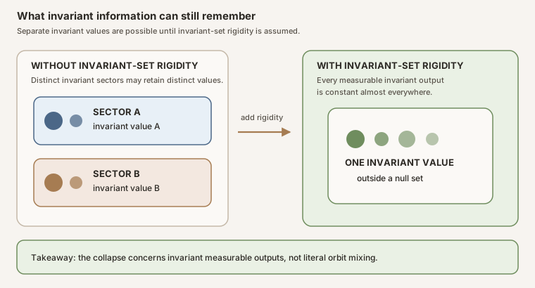
The second theorem removes that remaining component label. If every exactly invariant measurable event is trivial modulo null sets, an invariant measurable real function cannot separate two positive-mass invariant regions. It must be constant almost everywhere. That is the rigidity introduced here.
Only after identifying the constant may one say “space average.” On a finite measure that has not been normalized, the space average is not the raw integral. It is the integral divided by total mass. On a probability space, the total mass is one, so the distinction disappears.
This ordering prevents three common errors:
- treating invariant as synonymous with constant;
- calling an unnormalized integral an expectation; and
- dividing by total mass before proving that the mass is nonzero.
Learning objectives and reading paths
By the summit, a reader should be able to:
- distinguish
PreErgodic T μfromErgodic T μin Mathlib; - explain why the conditional-expectation representative is exactly invariant even though its constant identification is only almost everywhere;
- derive the normalization factor from an integral identity rather than from a probabilistic guess;
- read Mathlib’s
⨍ x, f x ∂μnotation and its totalized boundary behavior; - state all six public RMT-28 declarations with their true assumptions;
- explain why the finite-mass API takes an explicit proof
hμ : μ ≠ 0; - audit five compiled boundary models that prevent stronger hidden assumptions; and
- reproduce the warning-fatal build and the six axiom reports.
Fast path. Read the theorem ledger, the proof ladder, the five boundary probes, and the source-fidelity section.
Mathematical path. Read from the next section through the derivation of the constant, then work Exercises 1 through 15.
Lean path. Focus on the declaration-by-declaration sections, the private helper ledger, the exact code excerpts, and Exercises 16 through 20.
Pre-ergodicity is the rigidity core
Start with a measurable space \((\Omega,\mathcal F)\), a measure \(\mu\), and a map \(T:\Omega\to\Omega\). A measurable set \(S\) is exactly invariant when
\[ T^{-1}S=S. \]Mathlib collects those sets into MeasurableSpace.invariants T. The
definition uses literal equality of sets. It does not quotient sets by null
differences.
PreErgodic T μ asserts that every such set is constant as an event under the
almost-everywhere filter. Equivalently, every exactly invariant measurable
set is null or conull:
The prefix “pre” does not mean approximate or unfinished. It marks the
invariant-event rigidity without demanding that \(T\) preserve the measure.
Mathlib then defines Ergodic T μ by bundling two structures:
| Component | Meaning | Used here for |
|---|---|---|
MeasurePreserving T μ μ | \(T\) is measurable and its pushforward preserves \(\mu\) | Importing the RMT-27 time-average theorem |
PreErgodic T μ | Exactly invariant measurable events are null or conull | Collapsing invariant conditional expectation to a constant |
This split produces a stronger API because the conditional-expectation identification does not use measure preservation. A caller who already has pre-ergodic rigidity can use the first four public declarations without manufacturing an unused dynamical premise.
Prior work, contribution, and explicit nonclaims
Historical lineage. Birkhoff’s individual ergodic theorem is the historical source of the almost-everywhere time-average problem (Birkhoff 1931). RMT-28 does not claim to formalize the 1931 paper line by line. It specializes the repository’s already checked finite-measure theorem through current Mathlib interfaces.
Immediate formal predecessor. RMT-27 proves almost-everywhere convergence to conditional expectation on a finite measure-preserving system. It also explains exact invariant sigma algebras, representative transport, uniform integrability, and the finite-measure Vitali bridge. This chapter reuses that endpoint rather than repeating its proof.
This milestone’s contribution. The checked module contributes:
- a reusable pointwise invariance theorem for conditional expectation onto
MeasurableSpace.invariants T; - a private, assumption-minimal bridge from exact invariance and
PreErgodic T μto almost-everywhere constancy; - public identification of that constant as Mathlib’s integral average on a finite nonzero measure;
- explicit normalized-integral and probability presentations;
- two full-sequence Birkhoff corollaries that use full ergodicity only where RMT-27 needs measure preservation; and
- five executable boundary probes that freeze the intended assumptions.
Not claimed. The module proves no convergence rate, no everywhere convergence, no uniform convergence in the initial state, no mixing theorem, and no central limit theorem. It does not show that the exact invariant sigma algebra literally equals the trivial sigma algebra. It does not transfer ergodicity from \(T\) to a powered map \(T^b\). It proves no Kingman theorem, samplewise cocycle-growth limit, Lyapunov exponent, or Oseledets splitting. It assumes neither injectivity, surjectivity, nor invertibility.
Exact public theorem ledger
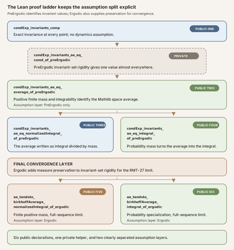
RMT-28 exposes six declarations. The first four concern the invariant conditional expectation itself. The final two combine that rigidity with RMT-27’s orbit convergence.
| No. | Declaration | Main assumptions | Conclusion |
|---|---|---|---|
| 1 | condExp_invariants_comp | none beyond ambient types | The selected representative is literally fixed by \(T\) |
| 2 | condExp_invariants_ae_eq_average_of_preErgodic | finite \(\mu\), μ ≠ 0, PreErgodic T μ, integrable \(f\) | Conditional expectation is almost everywhere ⨍ x, f x ∂μ |
| 3 | condExp_invariants_ae_eq_normalizedIntegral_of_preErgodic | same as 2 | The same target is \(\mu_{\mathbb R}(\Omega)^{-1}\int f\,d\mu\) |
| 4 | condExp_invariants_ae_eq_integral_of_preErgodic | probability \(\mu\), PreErgodic T μ, integrable \(f\) | The same target is \(\int f\,d\mu\) |
| 5 | ae_tendsto_birkhoffAverage_normalizedIntegral_of_ergodic | finite \(\mu\), μ ≠ 0, Ergodic T μ, integrable \(f\) | Full Birkhoff sequence converges almost everywhere to the normalized integral |
| 6 | ae_tendsto_birkhoffAverage_integral_of_ergodic | probability \(\mu\), Ergodic T μ, integrable \(f\) | Full Birkhoff sequence converges almost everywhere to \(\int f\,d\mu\) |
Three assumption distinctions control the theorem statements.
First, hμ : μ ≠ 0 is an explicit proposition in the finite-measure public
API. The proof installs the typeclass NeZero μ locally only where Mathlib’s
mass-cancellation lemma needs it. Callers see the mathematical boundary
directly.
Second, the conditional-expectation theorems require only PreErgodic. The
final orbit theorems require Ergodic, because they project both
hT.toPreErgodic and hT.toMeasurePreserving.
Third, integrability first enters when the constant is identified with an
integral. Exact invariance and the private existential constancy statement are
valid for Mathlib’s totalized conditional expectation even without
Integrable f μ.
Declaration 1: exact representative invariance
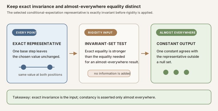
The first public declaration is deliberately stronger than an almost-everywhere equality:
theorem condExp_invariants_comp :
    (μ[f | MeasurableSpace.invariants T]) ∘ T =
      μ[f | MeasurableSpace.invariants T]
The proof has one conceptual step. Conditional expectation onto
MeasurableSpace.invariants T is strongly measurable for that sigma algebra.
Mathlib’s MeasurableSpace.comp_eq_of_measurable_invariants says that a
real-valued measurable function on this exact invariant sigma algebra is
fixed by composition with \(T\). The result concerns Mathlib’s selected total
representative, so it is a function equality at every point.
This theorem assumes no finiteness, nonzero mass, integrability, measure preservation, or pre-ergodicity. Those hypotheses do not participate in the representative-level fact.
The private hinge: constancy from PreErgodic
The source next introduces one nonpublic lemma:
private theorem condExp_invariants_ae_eq_const_of_preErgodic
    (hT : PreErgodic T μ) :
    ∃ c : ℝ, μ[f | MeasurableSpace.invariants T] =ᵐ[μ]
      fun _ : Ω ↦ c
Why keep it private? The existential constant is only an intermediate proof object. A downstream user wants the identified value, not an unnamed witness. Keeping the bridge private leaves the public API mathematical rather than tactic-shaped.
The proof feeds two facts to
PreErgodic.ae_eq_const_of_ae_eq_comp:
- the conditional-expectation representative is measurable on the ambient sigma algebra; and
- Declaration 1 gives exact equality after composition with \(T\).
The measurability conversion is worth reading carefully. Conditional
expectation is first strongly measurable on the smaller invariant sigma
algebra. The inclusion MeasurableSpace.invariants_le T lets Lean view it as
strongly measurable, hence measurable, on the ambient sigma algebra.
The conclusion is
\[ \exists c\in\mathbb R, \quad \mathbb E_\mu[f\mid\mathcal I_T](\omega)=c \quad\text{for almost every }\omega. \]No integral has yet appeared, and the value of \(c\) is still unknown.
Declaration 2: identify the constant as Mathlib’s average
The canonical public bridge is:
theorem condExp_invariants_ae_eq_average_of_preErgodic
    [IsFiniteMeasure μ]
    (hμ : μ ≠ 0) (hT : PreErgodic T μ) (hf : Integrable f μ) :
    μ[f | MeasurableSpace.invariants T] =ᵐ[μ]
      fun _ : Ω ↦ ⨍ x, f x ∂μ
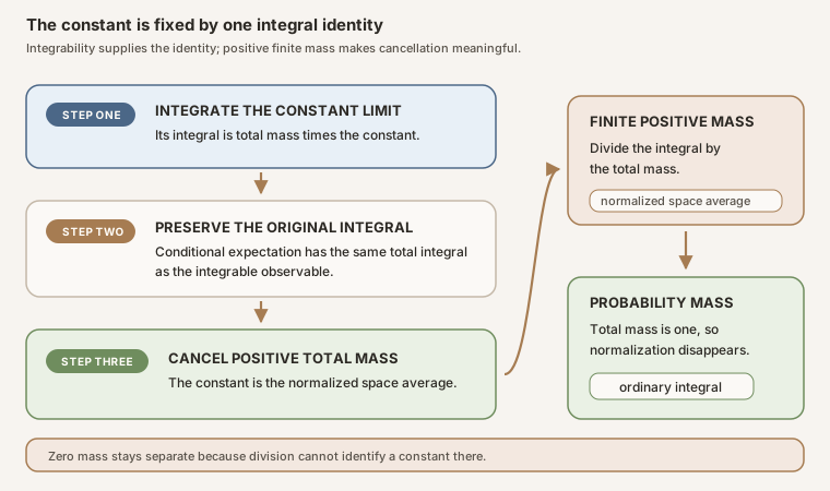
The proof first installs NeZero μ from the explicit proof hμ. It obtains
the private constant \(c\), then integrates the almost-everywhere equality.
The integral of the constant function is
The whole-space conditional-expectation identity gives
\[ \int_\Omega \mathbb E_\mu[f\mid\mathcal I_T]\,d\mu {} = \int_\Omega f\,d\mu. \]Combining the two equalities yields
\[ \mu_{\mathbb R}(\Omega)c {} = \int_\Omega f\,d\mu. \]Mathlib also proves
\[ \mu_{\mathbb R}(\Omega) \operatorname{Avg}_{\mu}(f) {} = \int_\Omega f\,d\mu \]for finite measures. Because hμ makes the real total mass nonzero, left
cancellation identifies \(c\) with ⨍ x, f x ∂μ.
This proof route avoids expanding an inverse immediately. It uses Mathlib’s average as the canonical middle object, delegates the normalization arithmetic to the library, and makes explicit where nonzero mass is used.
Mathlib’s ⨍ and the normalization ledger
Mathlib writes an integral average as:
⨍ x, f x ∂μ
For a real-valued function, average_eq rewrites it as
The notation is useful because it keeps three spaces separate:
| Measure regime | Total mass | Correct constant |
|---|---|---|
| Finite and nonzero | arbitrary positive finite mass | ⨍ x, f x ∂μ |
| Finite and nonzero, expanded | \(\mu_{\mathbb R}(\Omega)\) | \(\mu_{\mathbb R}(\Omega)^{-1}\int f\,d\mu\) |
| Probability | \(1\) | \(\int f\,d\mu\) |
The subscript \(\mathbb R\) reminds us that μ.real univ is a real-valued
mass obtained from the extended-nonnegative measure. Finiteness makes that
conversion faithful. Nonzeroness makes cancellation legitimate.
Why the integral average is totalized
Mathlib’s Bochner integral, conditional expectation, real inverse, and integral average are total functions. Their notation therefore continues to denote a term outside the regime where a textbook might leave it undefined.
For example, the real inverse satisfies \(0^{-1}=0\). The average of a function under the zero measure is zero. Almost-everywhere propositions under the zero measure are automatically true because every set is null. These choices are valuable for algebraic rewriting and theorem reuse, but they can erase information at a boundary.
The public RMT-28 finite-mass theorem therefore does not infer mathematical content merely because a normalized expression typechecks. It requires:
[IsFiniteMeasure μ], so total mass is finite;hμ : μ ≠ 0, so division and cancellation carry positive-mass meaning;hT : PreErgodic T μ, so invariant information is almost everywhere trivial; andhf : Integrable f μ, so the conditional-expectation integral identity carries the intended observable rather than a totalized fallback.
Declarations 3 and 4: two equivalent presentations
Declaration 3 exposes the finite-mass formula directly:
theorem condExp_invariants_ae_eq_normalizedIntegral_of_preErgodic
    [IsFiniteMeasure μ]
    (hμ : μ ≠ 0) (hT : PreErgodic T μ) (hf : Integrable f μ) :
    μ[f | MeasurableSpace.invariants T] =ᵐ[μ]
      fun _ : Ω ↦ (μ.real univ)⁻¹ * ∫ x, f x ∂μ
Its proof does not redo the integration argument. It specializes Declaration
2 and rewrites only average_eq and real scalar multiplication.
Declaration 4 specializes normalization to a probability measure:
theorem condExp_invariants_ae_eq_integral_of_preErgodic
    [IsProbabilityMeasure μ]
    (hT : PreErgodic T μ) (hf : Integrable f μ) :
    μ[f | MeasurableSpace.invariants T] =ᵐ[μ]
      fun _ : Ω ↦ ∫ x, f x ∂μ
IsProbabilityMeasure μ supplies finite mass and nonzeroness. Mathlib’s
average_eq_integral then removes the denominator because total mass is one.
The word “expectation” is appropriate only in this probability specialization. On a mass-two measure, the raw integral is twice the average. Calling both expressions expectation would conceal the normalization that the Lean interface makes explicit.
Declarations 5 and 6: return to orbit averages
The first four declarations concern the conditional-expectation target. They do not assert that finite-time orbit averages converge. Declarations 5 and 6 join the rigidity result to RMT-27.
The finite nonzero endpoint is:
theorem ae_tendsto_birkhoffAverage_normalizedIntegral_of_ergodic
    [IsFiniteMeasure μ]
    (hμ : μ ≠ 0) (hT : Ergodic T μ) (hf : Integrable f μ) :
    ∀ᵐ ω ∂μ,
      Tendsto (fun n ↦ birkhoffAverage ℝ T f n ω) atTop
        (nhds ((μ.real univ)⁻¹ * ∫ x, f x ∂μ))
The probability endpoint is:
theorem ae_tendsto_birkhoffAverage_integral_of_ergodic
    [IsProbabilityMeasure μ]
    (hT : Ergodic T μ) (hf : Integrable f μ) :
    ∀ᵐ ω ∂μ,
      Tendsto (fun n ↦ birkhoffAverage ℝ T f n ω) atTop
        (nhds (∫ x, f x ∂μ))
Both proofs use filter_upwards to intersect two conull events:
- RMT-27 gives convergence to conditional expectation using
hT.toMeasurePreservingandhf. - RMT-28 identifies that conditional expectation using
hT.toPreErgodicandhf.
At a point where both facts hold, simpa rewrites the target. The proof does
not repeat a maximal theorem, a Vitali argument, or conditional-expectation
uniqueness. The entire new mathematical burden is the ergodic rigidity and
normalization step.
Why full Ergodic belongs only here
Suppose a map has the null-or-conull property for exactly invariant sets but does not preserve \(\mu\). Its invariant conditional-expectation representative can still be rigid, because that statement concerns the invariant sigma algebra and the measure’s null sets. Yet finite-time orbit averages need not obey the measure-preserving Birkhoff theorem.
The public split records that distinction mechanically:
\[ \texttt{PreErgodic} \Longrightarrow \text{conditional-expectation rigidity}, \]while
\[ \texttt{Ergodic} {} = \texttt{MeasurePreserving}+\texttt{PreErgodic} \Longrightarrow \text{time-average convergence to the rigid target}. \]This is assumption minimization with mathematical content, not merely a Lean refactor.
Source-order declaration map
The six public declarations are best read as one dependency chain rather than as six restatements.
1. condExp_invariants_comp
This theorem produces literal representative invariance. Its body uses only
stronglyMeasurable_condExp and
MeasurableSpace.comp_eq_of_measurable_invariants.
Private bridge: condExp_invariants_ae_eq_const_of_preErgodic
This helper inserts PreErgodic T μ and concludes that the invariant
representative is almost everywhere some constant. It is private because the
constant is still unidentified.
2. condExp_invariants_ae_eq_average_of_preErgodic
This is the main identification proof. It consumes finite mass, explicit
nonzero measure, and integrability. It integrates the private equality, uses
the whole-space conditional-expectation identity, and cancels the real total
mass against Mathlib’s measure_smul_average theorem.
3. condExp_invariants_ae_eq_normalizedIntegral_of_preErgodic
This is a presentation corollary. It rewrites the integral average as inverse real mass times integral.
4. condExp_invariants_ae_eq_integral_of_preErgodic
This is the probability presentation. It obtains nonzero finite mass from the probability instance and rewrites Mathlib’s average as the ordinary integral.
5. ae_tendsto_birkhoffAverage_normalizedIntegral_of_ergodic
This is the finite nonzero orbit endpoint. It intersects RMT-27 convergence
with Declaration 3. The bundled Ergodic hypothesis supplies both projections
that those two branches need.
6. ae_tendsto_birkhoffAverage_integral_of_ergodic
This is the probability orbit endpoint. It intersects RMT-27 convergence with Declaration 4 and leaves the reader-facing limit as the ordinary integral.
No public theorem states convergence to Mathlib’s ⨍ notation directly. The
average remains the canonical conditional-expectation bridge, while the two
orbit endpoints expose the forms most useful to later formalization: explicit
finite-mass normalization and probability expectation.
Exact invariance is not a trivial sigma algebra identity
The proof relies on a subtle but essential distinction.
The exact invariant sigma algebra is a concrete measurable space built from sets satisfying \(T^{-1}S=S\). Even under pre-ergodicity, that sigma algebra need not be definitionally equal to the bottom sigma algebra. It may contain nonempty invariant null sets, complements of those sets, or other sets that are distinct as sets while representing trivial events modulo \(\mu\).
What pre-ergodicity says is measure-relative:
\[ S\in\mathcal I_T \Longrightarrow S={}^\mu\varnothing \quad\text{or}\quad S={}^\mu\Omega, \]where the superscript indicates equality almost everywhere. From that event statement, Mathlib derives the function statement that an invariant measurable real function is almost everywhere constant.
RMT-28 therefore proves this sequence:
\[ g\circ T=g \quad\text{pointwise}, \]then
\[ \exists c,\quad g={}^\mu (\omega\mapsto c). \]It does not rewrite MeasurableSpace.invariants T to a bottom measurable
space. That would be a stronger literal claim and is neither needed nor
proved.
Exact sets, completed events, and representatives
There are three nearby objects that should not be conflated:
- an exactly invariant measurable set \(S\), with \(T^{-1}S=S\);
- an event invariant only modulo a null set; and
- a chosen function representative that is pointwise fixed by composition.
Mathlib’s invariant sigma algebra in this module uses the first. Conditional expectation supplies a selected representative measurable for that sigma algebra, which yields the third. Pre-ergodicity then gives a conclusion modulo null sets. The proof crosses these levels through named lemmas rather than silently treating them as definitionally equal.
Why integrability enters only at identification
The selected conditional expectation is totalized. Its measurability for the
conditioning sigma algebra and the resulting exact composition identity are
available without Integrable f μ. The private pre-ergodic theorem can thus
show that this total function is almost everywhere some constant without
knowing whether \(f\) is integrable.
That broad statement has limited analytic content. To prove that the constant
is the space average of the original observable, the proof uses
setIntegral_condExp on the whole space. That theorem needs
Integrable f μ. The assumption is not decorative, and it is not inherited
from pre-ergodicity.
This is a useful formalization pattern:
- keep structural properties of totalized objects as general as the library supports;
- introduce analytic hypotheses exactly where their information is consumed; and
- expose a public theorem only when its statement reflects the intended mathematical regime.
The private boundary-support ledger
After the six public declarations, the source opens section BoundaryProbes.
The section contains fourteen private helpers before the five anonymous
examples. They are test infrastructure, not exported API.
| Source order | Private helper | Job in the probes |
|---|---|---|
| 1 | rmt28ConstantFalse | Defines the base map on Bool that sends both points to false |
| 2 | rmt28MassTwoDirac | Defines the finite nonprobability measure \(2\,\delta_{\mathrm{false}}\) |
| 3 | rmt28TwoAtomMeasure | Defines \(\delta_{\mathrm{false}}+\delta_{\mathrm{true}}\) |
| 4 | rmt28TwoAtomObservable | Defines the separator with value zero at false and one at true |
| 5 | rmt28ConstantFalse_not_injective | Proves the constant map is not injective |
| 6 | rmt28ConstantFalse_not_surjective | Proves true is not in the map’s range |
| 7 | rmt28ConstantFalse_measurePreserving_dirac | Computes the pushforward of \(\delta_{\mathrm{false}}\) and proves preservation |
| 8 | rmt28PreErgodic_dirac | Proves every map is pre-ergodic under a Dirac measure at any chosen support point |
| 9 | rmt28ConstantFalse_ergodic_dirac | Bundles helpers 7 and 8 into full ergodicity |
| 10 | rmt28ConstantFalse_not_measurePreserving_dirac_true | Proves the constant-false map moves a Dirac mass supported at true |
| 11 | rmt28MassTwoDirac_ne_zero | Proves the scaled Dirac measure is not zero by evaluating the whole space |
| 12 | private IsFiniteMeasure rmt28MassTwoDirac instance | Supplies finite mass for the scaled Dirac theorem |
| 13 | private IsFiniteMeasure rmt28TwoAtomMeasure instance | Supplies finite mass for the two-atom countermodel |
| 14 | rmt28ConstantFalse_ergodic_massTwoDirac | Transfers Dirac ergodicity through scalar multiplication by two |
Helper 8 is intentionally more general than the concrete constant map and
the support point false. A
Dirac measure sees only its supporting point. For any map \(S\), every event
is either true or false at that support, so it is automatically null or
conull. Measure preservation remains a separate question, answered for the
constant map by helper 7.
Helper 10 turns that separation into an executable witness. A Dirac mass at
true remains pre-ergodic under the constant-false map, but the map pushes its
mass to false and therefore does not preserve it.
Helper 11 deserves similar attention. The mass-two probe calls the public
finite theorem with an explicit proof that the measure is not zero. The test
does not rely on an ambient global NeZero instance, mirroring the public API
after canonization.
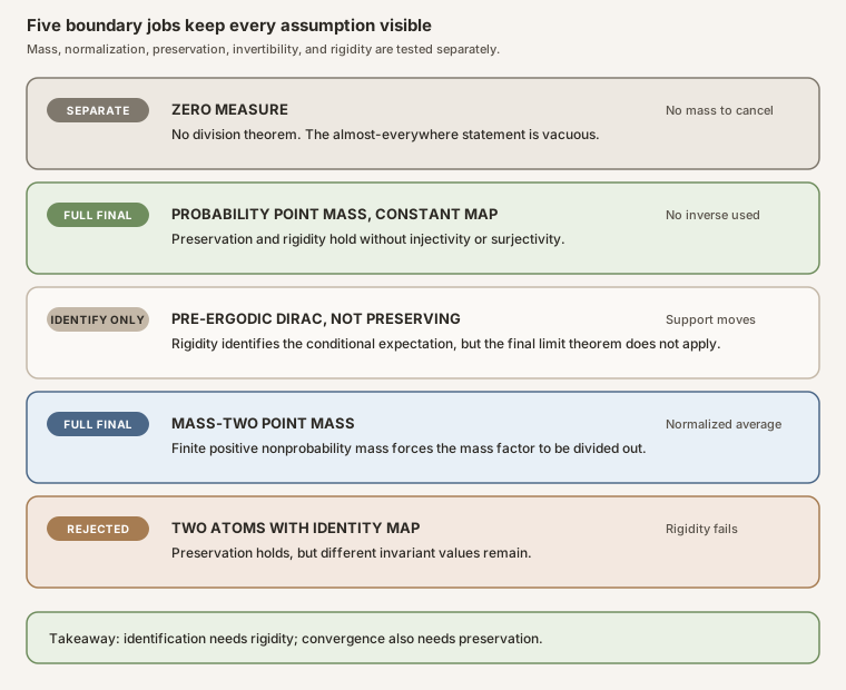
Anonymous probe 1: probability Dirac without bijectivity
The first example conjoins four facts about
It proves that \(T\) is ergodic, not injective, and not surjective. It then
quantifies over every integrable h : Bool → ℝ and invokes the probability
Birkhoff endpoint:
This model is small but decisive. Measure preservation concerns the
pushforward of the measure, not pointwise invertibility of the map. Since all
mass is concentrated at false and \(T(\mathrm{false})=\mathrm{false}\), the
pushforward is unchanged even though the unused point true has no preimage.
The theorem must therefore not demand injectivity, surjectivity, a measurable inverse, or a bijective measurable equivalence.
Anonymous probe 2: pre-ergodic without measure preservation
The second example moves the Dirac support from false to true while
keeping the same constant-false map:
The general Dirac helper proves PreErgodic T μ: every measurable event is
still null or conull under a one-point measure. Yet \(T\) moves the supporting
point from true to false, so its pushforward is
\(\delta_{\mathrm{false}}\), not \(\delta_{\mathrm{true}}\). The source proves
¬ MeasurePreserving rmt28ConstantFalse (Measure.dirac true)
  (Measure.dirac true)
and therefore cannot build Ergodic T μ.
Despite that failure, the probability conditional-expectation identification still applies:
\[ \mathbb E_{\delta_{\mathrm{true}}} [h\mid\mathcal I_T] {} = \int h\,d\delta_{\mathrm{true}} \quad\text{almost everywhere}. \]This probe is the direct witness for the weakened public API. Requiring full
Ergodic in Declaration 4 would demand measure preservation that its proof
does not use. The probe does not claim Birkhoff convergence, because that is
exactly the point where RMT-27 needs preservation.
Anonymous probe 3: mass two fixes the normalization
The third example returns to the Dirac mass at false and scales the measure:
Scalar multiplication preserves ergodicity, and the private finite-measure instance makes the general finite theorem available. The proof computes two quantities explicitly:
\[ \mu_{\mathbb R}(\Omega)=2, \qquad \int h\,d\mu=2h(\mathrm{false}). \]Hence
\[ \mu_{\mathbb R}(\Omega)^{-1}\int h\,d\mu {} = 2^{-1}\bigl(2h(\mathrm{false})\bigr) {} = h(\mathrm{false}). \]The anonymous theorem concludes almost-everywhere convergence to
h false, while repeating the proofs that the map is neither injective nor
surjective.
This probe catches a normalization bug that a probability-only test would miss. If the public finite theorem incorrectly targeted the raw integral, it would predict \(2h(\mathrm{false})\), not the orbit value \(h(\mathrm{false})\).
Anonymous probe 4: the zero measure is ergodic and vacuous
The fourth example uses the identity map and the zero measure. Mathlib proves
Ergodic.zero_measure measurable_id
so ergodicity alone does not imply positive mass. The same conjunction proves
that no NeZero (0 : Measure Bool) instance can exist, then discharges the
normalized almost-everywhere convergence proposition by simplification.
This is not evidence that an orbit has a meaningful zero average. There is no positive-mass initial state against which the assertion could fail. The almost-everywhere filter for the zero measure regards every predicate as true. At the same time, inverse zero and the zero-measure integral make the target expression reduce to zero.
These boundary facts support two design decisions:
- zero measure belongs to Mathlib’s general
Ergodicboundary; and - the meaningful finite normalized theorem must take
hμ : μ ≠ 0explicitly.
Anonymous probe 5: the weak gate is necessary
The fifth example uses
and the observable
\[ f(\mathrm{false})=0, \qquad f(\mathrm{true})=1. \]Every measurable set is invariant under the identity. The singleton \(\{\mathrm{false}\}\) and its complement both have positive mass, so the source proves the exact weak-gate failure
¬ PreErgodic id rmt28TwoAtomMeasure
and then derives
¬ Ergodic id rmt28TwoAtomMeasure
by projecting toPreErgodic from any hypothetical ergodicity proof. This
ordering matters. The conditional-expectation identification theorems assume
only PreErgodic, so a countermodel refuting only the stronger bundled
Ergodic premise would not isolate the necessary gate.
Because the invariant sigma algebra of the identity map is the full ambient sigma algebra, conditional expectation of the integrable separator is the separator itself almost everywhere. The source proves that this function cannot be almost everywhere constant: evaluating the equality at both atoms would force \(0=1\).
The anonymous result therefore proves that conditional expectation does not collapse to the normalized integral. This is a direct countermodel to dropping pre-ergodicity from Declarations 2 and 3.
Boundary matrix
| Model | Finite? | Nonzero? | Pre-ergodic? | Measure preserving? | Main lesson |
|---|---|---|---|---|---|
| \(\delta_{\mathrm{false}}\), constant map | yes | yes | yes | yes | Ergodicity does not imply bijectivity |
| \(\delta_{\mathrm{true}}\), constant-false map | yes | yes | yes | no | Conditional-expectation rigidity needs only pre-ergodicity |
| \(2\delta_{\mathrm{false}}\), constant map | yes | yes | yes | yes | The finite target needs total-mass normalization |
| zero measure, identity | yes | no | yes | yes | Ergodicity permits a vacuous zero-mass boundary |
| two equal atoms, identity | yes | yes | no | yes | Pre-ergodicity is necessary for collapse to one constant |
The last row is particularly informative. Measure preservation alone is not enough, even though RMT-27 still identifies the Birkhoff limit perfectly. Its target is the nonconstant observable itself.
Common wrong turns and why Lean rejects them
Replacing PreErgodic with Ergodic everywhere
That theorem would be true but needlessly strong. The conditional-expectation proof never projects measure preservation. The final source keeps the weaker rigidity structure until orbit convergence enters.
Calling the invariant sigma algebra literally trivial
Pre-ergodicity trivializes invariant events modulo the measure. Null invariant sets can remain distinct as sets, so literal sigma-algebra equality is not the proved statement.
Starting with an almost-everywhere invariance lemma
The selected conditional-expectation representative is exactly invariant. Using a weaker almost-everywhere route would discard structure and require a stronger quasi-measure-preserving interface to recover constancy. Declaration 1 makes the exact fact reusable.
Omitting integrability because conditional expectation is total
Totality guarantees a term, not the intended analytic identity. The proof
uses setIntegral_condExp with hf to connect the constant to the original
observable’s integral.
Cancelling mass without excluding zero
Real inversion is totalized, so the formula still parses at zero. Cancellation
does not. The explicit hμ : μ ≠ 0 marks the information boundary.
Using the raw integral on a nonprobability space
The mass-two Dirac probe refutes this immediately. The raw integral scales with total mass; the orbit average does not.
Requiring an inverse map
The probability and mass-two Dirac probes use a map that is neither injective nor surjective. The proof needs no inverse.
Transferring ergodicity to a powered map
Measure preservation passes to iterates, but ergodicity of \(T\) does not in general imply ergodicity of \(T^b\). A two-cycle is ergodic for one-step dynamics under its uniform probability measure, while its square is the identity and preserves each point. RMT-28 never asks for powered-map ergodicity.
Reading almost-everywhere convergence as everywhere convergence
The final declarations quantify with ∀ᵐ ω ∂μ. They permit a null exceptional
set and say nothing about a uniform convergence rate.
Source fidelity and proof authority
This chapter follows the checked module
NonlinearDynamics.Random.RandomCocycles.ErgodicBirkhoffLimit at
formalization/NonlinearDynamics/Random/RandomCocycles/ErgodicBirkhoffLimit.lean.
The source imports exactly:
import NonlinearDynamics.Random.RandomCocycles.PointwiseBirkhoffLimit
import Mathlib.Dynamics.Ergodic.Function
import Mathlib.MeasureTheory.Integral.Average
The exposition uses ordinary notation where it improves readability, but the translation ledger remains exact:
| Prose | Lean source |
|---|---|
| Exact invariant sigma algebra \(\mathcal I_T\) | MeasurableSpace.invariants T |
| Conditional expectation onto \(\mathcal I_T\) | `μ[f |
| Almost everywhere equality | =ᵐ[μ] |
| Integral average | ⨍ x, f x ∂μ |
| Real total mass | μ.real univ |
| Nonzero measure | explicit argument hμ : μ ≠ 0 |
| Pre-ergodic rigidity | PreErgodic T μ |
| Full ergodic system | Ergodic T μ |
| Full-sequence convergence | Tendsto from atTop to a neighborhood filter |
The phrase “positive finite mass” in the prose is shorthand for the combined
Lean assumptions [IsFiniteMeasure μ] and hμ : μ ≠ 0. For a measure, finite
and nonzero total mass yields strictly positive real total mass. The source
does not take a separate inequality hypothesis.
The phrase “probability expectation” refers only to declarations carrying
[IsProbabilityMeasure μ]. The finite nonprobability target is always called
an integral average or normalized integral.
Six axiom reports in source order
The module ends by printing axioms for every public declaration:
#print axioms condExp_invariants_comp
#print axioms condExp_invariants_ae_eq_average_of_preErgodic
#print axioms condExp_invariants_ae_eq_normalizedIntegral_of_preErgodic
#print axioms condExp_invariants_ae_eq_integral_of_preErgodic
#print axioms ae_tendsto_birkhoffAverage_normalizedIntegral_of_ergodic
#print axioms ae_tendsto_birkhoffAverage_integral_of_ergodic
Each report lists only:
propext
Classical.choice
Quot.sound
The private constancy lemma has no separate print command, but its dependencies
are included in the axiom report for the public average theorem that calls it.
There is no sorryAx, admit, or project-specific axiom.
How to run and inspect the proof
From the repository root, load Elan and compile the RMT-28 module directly:
source "$HOME/.elan/env"
cd formalization
lake env lean -DwarningAsError=true \
  NonlinearDynamics/Random/RandomCocycles/ErgodicBirkhoffLimit.lean
The command checks every declaration, all fourteen private boundary helpers, all five anonymous examples, and the six axiom reports.
Continue from formalization/ to build the complete project, then check the
public teaching content:
lake build

cd ..
make content-hygiene
make site-check
To preview this draft locally:
make blog-serve
The checked source remains authoritative if a rendered equation, line wrap, or explanatory paraphrase appears ambiguous.
Physics lens: time averages, ensemble averages, and equilibration
In statistical mechanics, \(\Omega\) is a phase space, \(T\) advances the microscopic state by one time step, and \(f\) is an observable such as a local energy, particle count in a region, or coarse macroscopic readout. The Birkhoff average asks what one indefinitely long trajectory reports:
\[ A_n f(\omega) {} = \frac1n\sum_{j=0}^{n-1} f(T^j\omega). \]The normalized space average asks what the measure-weighted ensemble reports:
\[ \operatorname{Avg}_{\mu}(f). \]RMT-27 says that a long trajectory retains exactly the invariant information available at its starting point. If phase space has two invariant regions of positive mass, a trajectory cannot cross between them, and their long-time values may differ. RMT-28 says that pre-ergodicity removes such a measurable positive-mass partition. The surviving invariant observable is then one constant outside a null set.
This does not prove physical equilibration in the stronger dynamical sense. The theorem gives no time scale, no monotone approach to equilibrium, no decay of correlations, and no mixing of distributions. A periodic cycle can be ergodic under its uniform measure while never resembling a randomizing process. Its time average can still converge to the ensemble average.
The distinction matters in nonlinear physics. Ergodic average identification answers a long-run equality question. Mixing answers how separated observations decorrelate. A central limit theorem answers the fluctuation scale around the limiting value. Large-deviation theory answers the probability of atypical finite-time averages. RMT-28 proves only the first.
A finite cycle computed by hand
Let \(\Omega=\{a,b,c\}\), let \(T\) cycle \(a\mapsto b\mapsto c\mapsto a\), and give each point mass \(w\gt0\). The total mass is \(3w\). For values \(f(a)=p\), \(f(b)=q\), and \(f(c)=r\), every orbit repeats the same three observations, only with a different initial phase. Hence
\[ A_n f(\omega) \longrightarrow \frac{p+q+r}{3}. \]The raw integral is
\[ \int f\,d\mu=w(p+q+r), \]while the normalized space average is
\[ (3w)^{-1}w(p+q+r) {} = \frac{p+q+r}{3}. \]The scale \(w\) cancels. This is the same normalization tested formally by the mass-two Dirac probe. If \(w=1/3\), the measure is a probability measure and the raw integral already equals the average.
Why this matters for random cocycles
Later random-matrix and random-cocycle milestones will study quantities built along an ergodic base orbit. Additive observables can use the theorem here directly. Matrix-growth quantities such as logarithms of product norms are typically subadditive rather than additive, so RMT-28 is not yet Kingman’s theorem and does not yet construct a Lyapunov exponent.
The value of this milestone is architectural. It fixes the normalization, the exact role of ergodicity, and the zero-measure boundary before those ideas enter a more difficult subadditive proof.
Solved exercises
Exercise 1: identify what RMT-27 leaves variable
What can the RMT-27 target remember on a nonergodic system?
Solution. It can remember any information measurable with respect to the exact invariant sigma algebra. Concretely, it may take different values on different positive-mass invariant components. RMT-27 identifies the target as conditional expectation onto that information; it does not force a global constant.
Exercise 2: separate PreErgodic from Ergodic
State the extra structure carried by Ergodic T μ.
Solution. PreErgodic T μ supplies the null-or-conull property for
exactly invariant measurable sets. Ergodic T μ extends it with
MeasurePreserving T μ μ. The conditional-expectation rigidity uses the
first component; the Birkhoff convergence endpoint uses both.
Exercise 3: test an invariant event
If \(S\) is exactly invariant and hT : PreErgodic T μ, what are the two
measure-theoretic possibilities?
Solution. Either \(\mu(S)=0\) or \(\mu(S^{\mathsf c})=0\). Equivalently, membership in \(S\) is almost everywhere false or almost everywhere true.
Exercise 4: distinguish two equalities
Which RMT-28 equality is pointwise, and which is only almost everywhere?
Solution. Declaration 1 proves the selected conditional-expectation representative satisfies \(g\circ T=g\) as literal function equality. The private pre-ergodic helper proves \(g=c\) only almost everywhere. A null set may retain exceptional representative values.
Exercise 5: explain why the invariant sigma algebra need not be bottom
Why does pre-ergodicity not imply literal equality with the bottom sigma algebra?
Solution. Pre-ergodicity trivializes invariant events only modulo null sets. An invariant null set can be nonempty and remain a distinct member of the exact invariant sigma algebra. Its event class is trivial for \(\mu\), but the set itself is not literally empty.
Exercise 6: derive the integral equation for the constant
Suppose \(g=c\) almost everywhere and \(g\) is the invariant conditional expectation of \(f\). Derive the equation that identifies \(c\).
Solution. Almost-everywhere equality gives \(\int g\,d\mu=\int c\,d\mu=\mu_{\mathbb R}(\Omega)c\). The whole-space conditional-expectation identity gives \(\int g\,d\mu=\int f\,d\mu\). Therefore \(\mu_{\mathbb R}(\Omega)c=\int f\,d\mu\).
Exercise 7: locate the nonzero-mass use
Where does hμ : μ ≠ 0 first become mathematically necessary?
Solution. It is not needed for exact invariance or existential constancy.
It is needed when the proof cancels μ.real univ to identify the unnamed
constant with the average. At zero mass the multiplication equation carries
no information about \(c\).
Exercise 8: compute a mass-four average
Let a finite measure have real total mass \(4\) and let \(\int f\,d\mu=12\). What constant does Declaration 3 identify?
Solution. The normalized target is \(4^{-1}\cdot12=3\). The raw integral \(12\) would be the wrong orbit-average target unless the measure were probability normalized.
Exercise 9: simplify the probability case
Why does Declaration 4 have no explicit nonzero argument?
Solution. IsProbabilityMeasure μ gives \(\mu(\Omega)=1\), hence finite
and nonzero mass. Mathlib supplies the corresponding instances, and
average_eq_integral rewrites the normalized average to the ordinary
integral.
Exercise 10: interpret totalization at zero
What does the normalized formula evaluate to under the zero measure, and why does that not establish a meaningful orbit law?
Solution. The integral is zero, the real total mass is zero, and the totalized inverse of zero is zero, so the expression is zero. Every almost-everywhere proposition under the zero measure is true, leaving no positive-mass initial state that tests the claim. The statement is valid but vacuous.
Exercise 11: isolate the weakened API witness
Why is the constant-false map with Measure.dirac true a useful model?
Solution. Any map is pre-ergodic for a Dirac measure, because only the
support point matters to null sets. The constant-false map moves the support
from true to false, so it is not measure preserving. The
conditional-expectation identification still holds, proving that full ergodicity would be
an unnecessary premise there.
Exercise 12: audit the nonbijective ergodic model
Why can the constant-false map be ergodic for Measure.dirac false?
Solution. It fixes the only point seen by the measure, so the pushforward
Dirac measure is unchanged. Dirac support also makes every exactly invariant
event null or conull. These two facts give ergodicity even though the map
collapses both Boolean points and never reaches true.
Exercise 13: compute the mass-two model
For \(\mu=2\delta_{\mathrm{false}}\), compute the normalized integral of an observable \(h\).
Solution. The real total mass is \(2\), and the integral is \(2h(\mathrm{false})\). Multiplying by \(2^{-1}\) yields \(h(\mathrm{false})\), exactly the value seen along the supported orbit.
Exercise 14: show the two-atom identity is not pre-ergodic
Which invariant event witnesses failure?
Solution. The singleton \(\{\mathrm{false}\}\) is exactly invariant under
the identity. It has mass one, and its complement also has mass one. It is
neither null nor conull, contradicting PreErgodic.
Exercise 15: show why the two-atom conditional expectation cannot collapse
Why is the separator \(f(\mathrm{false})=0\), \(f(\mathrm{true})=1\) not almost everywhere constant?
Solution. Both atoms have positive mass, so an almost-everywhere equality to a constant \(c\) must hold at both. That would give \(0=c\) and \(1=c\), hence \(0=1\), a contradiction. Under identity dynamics the invariant sigma algebra is full, so conditional expectation returns this separator almost everywhere.
Exercise 16: audit Declaration 1’s assumptions
Which of finiteness, nonzero mass, integrability, pre-ergodicity, and measure
preservation occur in condExp_invariants_comp?
Solution. None occur. The theorem is a structural property of the selected conditional expectation onto the exact invariant sigma algebra. Adding any of those assumptions would weaken the reusable interface.
Exercise 17: follow the two projections of Ergodic
Where does Declaration 5 send hT.toMeasurePreserving and
hT.toPreErgodic?
Solution. hT.toMeasurePreserving goes to RMT-27’s
ae_tendsto_birkhoffAverage_condExp. hT.toPreErgodic goes to RMT-28’s
condExp_invariants_ae_eq_normalizedIntegral_of_preErgodic. The proof
intersects the two conull events and rewrites the target.
Exercise 18: justify the private constancy helper
Why not expose condExp_invariants_ae_eq_const_of_preErgodic as the main
result?
Solution. Its existential witness has not been identified. Downstream mathematics needs the normalized integral, not an arbitrary constant chosen by a rigidity lemma. Keeping the helper private reduces API surface while the three public identification theorems expose useful canonical targets.
Exercise 19: refute powered-map ergodicity
Give an ergodic map whose square is not ergodic.
Solution. Let \(T\) swap two atoms carrying the uniform probability measure. Its only one-step invariant events are null or conull, so it is ergodic. But \(T^2=\operatorname{id}\), and each singleton is then invariant with probability \(1/2\), so the square is not pre-ergodic. RMT-28 correctly makes no powered-map claim.
Exercise 20: state the final probability theorem without overclaiming
Give its assumptions, conclusion, and three things it does not provide.
Solution. On a probability space, if hT : Ergodic T μ and
hf : Integrable f μ, then for \(\mu\)-almost every \(\omega\), the full
sequence birkhoffAverage ℝ T f n ω tends to \(\int f\,d\mu\) as
\(n\to\infty\). It does not provide convergence at every point, a convergence
rate, or mixing. It also makes no invertibility or powered-map ergodicity
claim.
Discussion
Everything in this section is interpretation of the checked theorem rather than an additional result. The warning-fatal declarations and boundary probes stand on their own; the broader lessons below would need separate formal or scientific tests if turned into new claims.
RMT-28 makes explicit the structure behind a familiar one-line formula. “Time average equals space average” requires a convergence theorem, an invariant-information target, a rigidity theorem, an integral identification, a nonzero denominator, and a normalization convention. Lean does not permit those layers to merge through familiarity alone.
The final canonization also illustrates why assumption minimization matters.
The first draft shape could have placed full Ergodic on every identification
theorem. The Dirac-at-true boundary model instantiates
conditional-expectation rigidity when measure preservation fails, so full
Ergodic would exclude a valid case. Full ergodicity becomes necessary only
when a claim about orbit averages imports RMT-27.
For physics, the theorem identifies an asymptotic value without describing the rate or path of convergence. A future quantitative theory might add mixing rates, spectral gaps, concentration, or fluctuation laws. None follows from this module. Keeping those questions separate protects later work from treating an existence theorem as a mechanism or time-scale theorem.
The next ridge
The additive ergodic endpoint is now explicit for both finite positive mass and probability normalization. The random-cocycle program can reuse its assumption ledger, but it cannot replace subadditive analysis with this corollary.
Kingman’s theorem must control a family satisfying a subadditive composition law rather than one additive observable. A samplewise matrix-growth limit then needs a precise link between cocycle products and that subadditive process. Lyapunov exponents and Oseledets splittings require further integrability, measurability, invariant-subspace, and multiplicative structure. Those remain later milestones.
RMT-29 now takes the next checked step: it combines the RMT-28 probability-integral Birkhoff endpoint with finite phase averaging to prove the upper limsup bound for nonnegative subadditive processes. It still makes no lower-bound or samplewise-convergence claim.
References
George D. Birkhoff. Proof of the Ergodic Theorem, Proceedings of the National Academy of Sciences 17(12), 656-660, 1931. This is the historical source of the individual ergodic theorem. RMT-28 is a modern Lean specialization built on the repository’s RMT-27 theorem, not a line-by-line formalization of Birkhoff’s paper.
This project. What the Orbit Remembers: Identifying the Birkhoff Limit in Lean, RMT-27. This checked predecessor proves finite-measure almost-everywhere convergence to conditional expectation onto the exact invariant sigma algebra.
Mathlib contributors.
Ergodic and pre-ergodic maps,
Mathlib 4.32.0. The pinned source defines PreErgodic through exactly
invariant events and defines Ergodic by adjoining measure preservation.
Mathlib contributors.
Functions invariant under an ergodic map,
Mathlib 4.32.0. RMT-28 uses
PreErgodic.ae_eq_const_of_ae_eq_comp for the private rigidity bridge.
Mathlib contributors.
Integral averages,
Mathlib 4.32.0. This pinned module defines ⨍, proves average_eq,
measure_smul_average, and the probability rewrite average_eq_integral.
Mathlib contributors.
Invariant sigma algebras,
Mathlib 4.32.0. The exact invariant-space interface supplies
MeasurableSpace.comp_eq_of_measurable_invariants and
MeasurableSpace.invariants_le.
This project.
NonlinearDynamics.Random.RandomCocycles.ErgodicBirkhoffLimit, RMT-28. The
warning-fatal Lean module is the authority for the six public declarations,
one private constancy bridge, fourteen private boundary helpers, five
anonymous probes, theorem assumptions, normalization, and six axiom reports
explained in this chapter.