
Milestone status. RMT-27’s Lean implementation is warning-fatal clean and
adds no axiom class beyond the standard Mathlib footprint
propext, Classical.choice, and Quot.sound. The prose and figures are
published as part of this open working note while human review remains pending.
For a slower ascent with a fully computed finite model, read Birkhoff Limits, Invariant Sigma Algebras, and Conditional Expectation. The reusable definitions are the invariant sigma algebra , conditional expectation , and uniform integrability .
The question RMT-26 left open
RMT-26 established an existence statement:
\[ \text{for almost every }\omega, \quad \exists c_\omega\in\mathbb R, \quad A_nf(\omega)\longrightarrow c_\omega. \]That theorem explicitly excludes a stronger conclusion. An existential witness selected separately at each point is not yet a measurable function. Even if one writes \(c(\omega)\), nothing in the bare statement says that \(c\) is integrable, invariant, or characterized by integrals. Those properties cannot be obtained merely by renaming the witness.
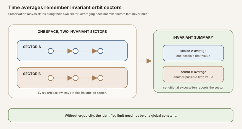
The difference is scientifically important. A trajectory in a nonlinear system can remain forever in one invariant component. Its time average can forget the initial phase within that component while retaining the component itself. If two components have different average energies, populations, or finite-time growth observables, one global number discards real dynamical information.
The target must therefore answer two questions at once:
- Which measurable information can an infinitely long orbit retain?
- Which integrable function is uniquely determined by that information and the original observable’s averages on every retained event?
The invariant sigma algebra answers the first question. Conditional expectation answers the second.
Prior work, contribution, and explicit nonclaims
Historical origin. Birkhoff’s 1931 paper established the individual ergodic theorem in a volume-preserving flow setting and sharply separated pointwise behavior from convergence in the mean (Birkhoff 1931). It is the historical origin of the pointwise question, not the exact source of the modern Lean interface used here.
Identification lineage. Chacon’s 1962 paper is explicitly devoted to the identification of limits of operator averages (Chacon 1962). Its title alone records an essential lesson: proving convergence and identifying the limit are separate proof stages. We use it as historical lineage, not as a claim that RMT-27 is a line-for-line formalization of Chacon’s operator framework.
Closest modern theorem shape. Hess, Seri, and Choirat state their Theorem 1 on a stationary probability space without assuming ergodicity. Their target is conditional expectation onto the invariant sigma field, and their paper also distinguishes exact invariant sets from almost-sure invariant sets and their completion (Hess, Seri, and Choirat 2010). Their theorem allows quasi-integrable extended-real observables, while RMT-27 treats real integrable observables. RMT-27 uses finite, not necessarily normalized, measure and follows the exact APIs in pinned Mathlib. The results are close in shape but not identical in scope or proof packaging.
Repository contribution. RMT-27 supplies a checked bridge from the RMT-26 convergence event to Mathlib conditional expectation. The new contribution is the complete formal chain:
- one total limit representative with a shift-stable fallback;
- exact invariant-sigma-algebra measurability for a strong representative;
- almost-everywhere transport between observable representatives;
- identical distribution and uniform integrability of orbit translates;
- uniform integrability of the Birkhoff averages;
- integrability and \(L^1\) convergence of the chosen limit;
- invariant-set integral identities without an inverse map; and
- conditional-expectation uniqueness for the original integrable observable.
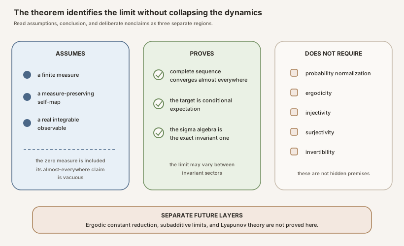
Nonclaims. The module does not prove that the limit is constant. It does not divide by \(\mu(\Omega)\), assume positive total mass, or specialize to a probability space. It does not prove an infinite-measure theorem, uniform pointwise convergence, convergence at every state, Kingman’s subadditive ergodic theorem, a Lyapunov exponent, or an Oseledets splitting.
What time averages retain
Let \(\mathcal I_T\) contain the measurable sets \(S\) satisfying \(T^{-1}S=S\) literally. If \(\omega\in S\), then \(T\omega\in S\), and the entire forward orbit remains in \(S\). Membership in \(S\) is information that the dynamics never erase.
An \(\mathcal I_T\)-measurable function can vary between invariant sectors but cannot vary in a way that distinguishes points after one application of the base map. For real-valued measurable functions, Mathlib’s invariant-space API connects the two descriptions:
\[ g\text{ is }\mathcal I_T\text{-measurable} \quad\Longrightarrow\quad g\circ T=g. \]The chosen Birkhoff limit will satisfy this equality pointwise. Conditional expectation then finds the unique integrable invariant-information function whose integral over every invariant event agrees with the integral of \(f\).
A finite nonprobability model
Take four states \(a_0,a_1,b_0,b_1\). Let \(T\) swap \(a_0\) with \(a_1\) and swap \(b_0\) with \(b_1\). Give the first orbit weights \(2,2\) and the second orbit weights \(1,1\). The total mass is \(6\), so this is not a probability measure. Equal weights within each two-cycle make \(T\) measure preserving.
Choose the observable:
| State | Measure weight | \(f\) | Long orbit average |
|---|---|---|---|
| \(a_0\) | \(2\) | \(1\) | \(3\) |
| \(a_1\) | \(2\) | \(5\) | \(3\) |
| \(b_0\) | \(1\) | \(-2\) | \(1\) |
| \(b_1\) | \(1\) | \(4\) | \(1\) |
Every orbit alternates within one row pair. The first pair averages to \((1+5)/2=3\), while the second averages to \((-2+4)/2=1\). The invariant sigma algebra can distinguish the two cycles, so the conditional expectation is \(3\) on the first and \(1\) on the second.
The normalized global integral is instead
\[ \frac{\int f\,d\mu}{\mu(\Omega)} {} = \frac{2\cdot1+2\cdot5-2+4}{6} {} = \frac73. \]Neither orbit has long-run average \(7/3\). This small model simultaneously explains why the general target need not be constant, why probability normalization is absent, and why ergodicity is an additional rigidity premise rather than a hidden part of the pointwise theorem.
Exact theorem and assumption ledger
The final Lean declaration is:
theorem ae_tendsto_birkhoffAverage_condExp
    [IsFiniteMeasure μ]
    (hT : MeasurePreserving T μ μ) (hf : Integrable f μ) :
    ∀ᵐ ω ∂μ,
      Tendsto (fun n ↦ birkhoffAverage ℝ T f n ω) atTop
        (nhds (μ[f | MeasurableSpace.invariants T] ω))
The assumptions mean exactly:
| Item | Present? | Role |
|---|---|---|
| Finite total measure | yes | Used by RMT-26 convergence and the finite-measure Vitali step |
| Measure preservation | yes | Propagates laws, integrability, and invariant-set restrictions along iterates |
| Real integrability | yes | Supplies an almost-everywhere strongly measurable representative and finite first moment |
| Probability normalization | no | The total mass may be \(0\), \(2\), or any finite value |
| Ergodicity | no | The target may remain nonconstant across invariant sectors |
| Injectivity or surjectivity | no | The restriction proof uses preimages and pushforward measures, not an inverse |
| Invertibility | no | Only forward iterates appear |
| Positive total mass | no | No division by \(\mu(\Omega)\) occurs |
The average at horizon zero is totalized by Mathlib. It plays no role in a tail limit, and the invariant-set integral identity is correctly stated only for \(n\ne0\).
Declarations 1 through 4: one total limit
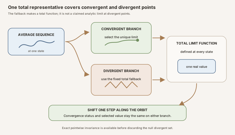
The first declaration is not an existential choice at each point. It is one function:
def birkhoffLimit (T : Ω → Ω) (f : Ω → ℝ) (ω : Ω) : ℝ :=
  limUnder atTop (fun n ↦ birkhoffAverage ℝ T f n ω)
Filter.limUnder returns the genuine limit when one exists. On a nonempty
codomain it also supplies a fixed fallback when no limit exists. The fallback
is not claimed to have mathematical meaning. Its purpose is to make
birkhoffLimit T f a total function that can be tested for measurability and
invariance.
Declarations 2 and 3 connect the total representative to convergence:
tendsto_birkhoffAverage_birkhoffLimit_of_existsconsumes an explicit finite limit witness;tendsto_birkhoffAverage_birkhoffLimit_of_memconsumes membership in the RMT-26 convergence event.
Declaration 4, birkhoffLimit_apply_base, is the pointwise identity needed
for invariance:
There are two branches. If the averages converge at \(\omega\), the prefix-shift
theorem says that they converge to the same value at \(T\omega\). If they do
not converge at \(\omega\), the reverse prefix-shift theorem proves that they
cannot converge at \(T\omega\) either. Both calls to limUnder therefore use
the same fallback. Literal invariance holds at every point, not only almost
everywhere.
Declarations 5 through 8: measurability and representative safety
Declaration 5, stronglyMeasurable_birkhoffLimit, says that measurable
dynamics and a strongly measurable observable produce a strongly measurable
total limit on the ambient sigma algebra. Each finite average is measurable,
and Mathlib’s StronglyMeasurable.limUnder packages the pointwise limit
constructor.
Declaration 6, measurable_birkhoffLimit_invariants, strengthens the domain
sigma algebra. It combines ambient measurability with the exact equality
\(L_f\circ T=L_f\) and concludes measurability for
MeasurableSpace.invariants T.
Declaration 7, ae_tendsto_birkhoffAverage_birkhoffLimit, imports the full
RMT-26 theorem and replaces its unnamed existential limit by the single total
representative:
Declaration 8, birkhoffLimit_ae_eq_of_ae_eq, protects the construction from
the choice of an \(L^1\) representative. If \(f=g\) almost everywhere and
\(T\) is quasi-measure preserving, every finite orbit average of \(f\) equals
the corresponding average of \(g\) almost everywhere. Applying limUnder
pointwise gives \(L_f=L_g\) almost everywhere.
This is the right interface boundary. A raw integrable function need not be ordinarily strongly measurable, but it has a strongly measurable version. We may reason exactly about that version and then transport the conclusion back without treating quotient representatives as definitionally equal.
Why pointwise convergence cannot pass integrals
Consider on \([0,1]\) the sequence
\[ u_n(x)=n\,\mathbf 1_{(0,1/n)}(x). \]For every \(x\gt0\), eventually \(x\notin(0,1/n)\), while \(u_n(0)=0\) for every \(n\). Thus \(u_n(x)\to0\) at every point. Nevertheless,
\[ \int_0^1 u_n(x)\,dx=1 \]for every \(n\). Almost-everywhere convergence alone does not force integrals to converge. The mass can concentrate into taller and narrower spikes.
The RMT-27 invariant-set argument must therefore rule out concentration in the Birkhoff averages. Dominated convergence is not available because there is no single integrable pointwise dominator for every average. The correct substitute is uniform integrability.
Declarations 9 through 13: identical laws, uniform integrability, and Vitali
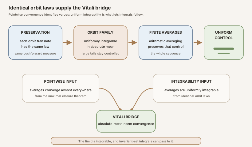
Declaration 9, identDistrib_orbit_iterate, is deliberately general. It
requires only that \(f\) be almost-everywhere measurable and that \(T\)
preserve \(\mu\). For every \(i\),
The proof compares pushforward measures. It needs no finite-measure premise.
Declaration 10, uniformIntegrable_orbit_iterate, adds finite mass and
integrability. Identical distribution transfers the same \(L^1\) tail control
to every orbit translate. Declaration 11,
uniformIntegrable_birkhoffAverage, applies Mathlib’s averaging theorem to
show that their Cesaro averages are uniformly integrable too.
Uniform integrability says, operationally, that no member of the family can hide a significant amount of absolute integral on an arbitrarily small measurable set. It is exactly the condition violated by the spike sequence.
Declaration 12, integrable_birkhoffLimit, combines uniform integrability with
the almost-everywhere convergence from declaration 7. Mathlib concludes that
the total limit is integrable. Declaration 13,
tendsto_L1_birkhoffAverage_birkhoffLimit, invokes the finite-measure Vitali
theorem and proves
This is strictly more than the RMT-26 pointwise conclusion and precisely what allows set integrals to pass to the limit.
Declarations 14 through 16: invariant-set integrals
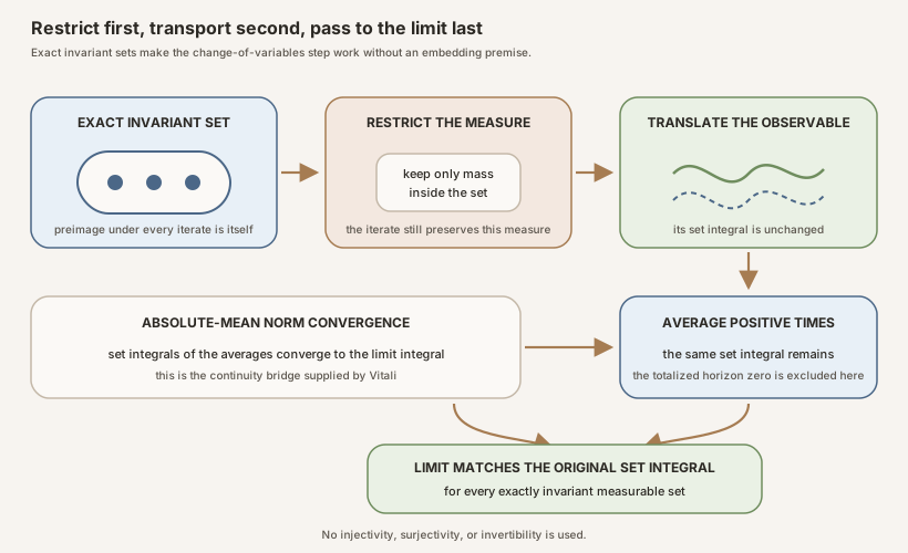
Let \(S\in\mathcal I_T\). Because \(T^{-1}S=S\), every iterate satisfies
\((T^i)^{-1}S=S\). Declaration 14,
setIntegral_orbit_iterate_eq, proves
The proof does not change variables through an inverse. It applies
MeasurePreserving.restrict_preimage, rewrites the preimage restriction using
exact invariance, and applies the pushforward integral theorem on
\(\mu\vert_S\). This remains valid for a noninjective map.
Declaration 15, setIntegral_birkhoffAverage_eq, sums the orbit identities
and divides by the positive horizon:
The nonzero premise is real information. At \(n=0\), the totalized average is zero, so the displayed identity would generally be false.
Declaration 16, setIntegral_birkhoffLimit_eq, uses \(L^1\) convergence to
pass the identity to the limit:
Declarations 17 and 18: conditional expectation and the summit
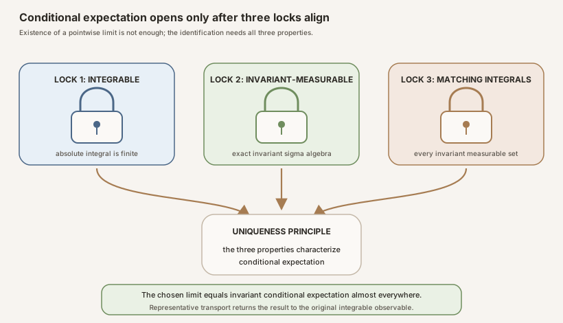
Conditional expectation onto \(\mathcal I_T\) is characterized by three locks. A candidate \(g\) must be:
- measurable with respect to invariant information;
- integrable; and
- equal to \(f\) after integration over every invariant measurable set.
For a strongly measurable version of \(f\), declarations 6, 12, and 16 open
those locks. The module’s private core invokes
ae_eq_condExp_of_forall_setIntegral_eq. Declaration 17,
birkhoffLimit_ae_eq_condExp, then returns to the original integrable
observable by using declaration 8 and condExp_congr_ae:
Declaration 18, ae_tendsto_birkhoffAverage_condExp, combines this equality
with declaration 7. It is the final full-sequence theorem.
Exact invariance versus invariance modulo null sets
Mathlib defines MeasurableSpace.invariants T using literal set equality
\(T^{-1}S=S\). A completed invariant sigma field may also include sets whose
preimages agree only modulo a null set. Those objects are closely related but
not definitionally identical.
Hess, Seri, and Choirat explicitly note this distinction: their invariant sets form a sigma field \(\mathcal I\), while almost-sure invariant sets form its probability completion. RMT-27 bridges the formal boundary by constructing an exactly invariant, exactly measurable representative for the internal strong version and then returning to the original observable through almost-everywhere equality. It does not silently replace exact invariance with completed invariance.
Another asymmetry matters. Mathlib proves
\[ \mathcal I_T\subseteq\mathcal I_{T^i}, \]because a set fixed by one step is fixed by every iterate. The converse is false in general: \(T^i\) can preserve periodic phase classes that one step of \(T\) swaps. The proof uses this inclusion only in the valid direction.
Declaration map in source order
| No. | Lean declaration | Mathematical role |
|---|---|---|
| 1 | birkhoffLimit | One total limUnder representative |
| 2 | tendsto_birkhoffAverage_birkhoffLimit_of_exists | Existing finite limit converges to the representative |
| 3 | tendsto_birkhoffAverage_birkhoffLimit_of_mem | Convergence-event membership gives the same conclusion |
| 4 | birkhoffLimit_apply_base | Literal one-step invariance, including fallback |
| 5 | stronglyMeasurable_birkhoffLimit | Ambient strong measurability for strong data |
| 6 | measurable_birkhoffLimit_invariants | Exact invariant-sigma-algebra measurability |
| 7 | ae_tendsto_birkhoffAverage_birkhoffLimit | RMT-26 convergence to the named representative |
| 8 | birkhoffLimit_ae_eq_of_ae_eq | Representative transport through all finite averages |
| 9 | identDistrib_orbit_iterate | Every orbit translate has the same law |
| 10 | uniformIntegrable_orbit_iterate | Uniform integrability of orbit observations |
| 11 | uniformIntegrable_birkhoffAverage | Uniform integrability survives Cesaro averaging |
| 12 | integrable_birkhoffLimit | The pointwise limit is integrable |
| 13 | tendsto_L1_birkhoffAverage_birkhoffLimit | Full-sequence convergence in \(L^1\) |
| 14 | setIntegral_orbit_iterate_eq | Orbit integrals agree on exact invariant sets |
| 15 | setIntegral_birkhoffAverage_eq | Positive-time average integrals agree |
| 16 | setIntegral_birkhoffLimit_eq | The limit inherits the invariant-set identities |
| 17 | birkhoffLimit_ae_eq_condExp | The named limit equals conditional expectation almost everywhere |
| 18 | ae_tendsto_birkhoffAverage_condExp | Final finite-measure pointwise theorem with identified target |
The private helper
birkhoffLimit_ae_eq_condExp_of_stronglyMeasurable isolates the exact
measurability proof. It is intentionally not part of the public API because
the useful theorem needs only Integrable f μ.
Five compiled boundary probes
The module freezes five adversarial examples beside the theorem.
- Zero measure. The almost-everywhere conclusion is vacuous, and no
NeZero μpremise appears. - Identity dynamics. The theorem applies without ergodicity.
- Nonergodic mass-two system. The identity on two atoms with measure
dirac false + dirac trueis proved not ergodic. Its total mass is two, so probability normalization is genuinely absent. - Full target on that system. The two-atom example retains the complete conditional-expectation target rather than replacing it by a constant.
- Noninvertible Dirac system. A constant map on
Boolpreservesdirac falsewhile being neither injective nor surjective, and the final theorem still applies.
These probes are not decorative examples. They prevent later refactors from quietly adding probability, ergodicity, invertibility, or positive-mass assumptions.
Proof engineering and common failure modes
Choosing unrelated limits
Selecting a separate witness from every existential convergence proof makes
measurability hard to state. birkhoffLimit provides one total function.
Ignoring the divergent branch
An invariant function must be defined and invariant at every point. The fallback branch is proved shift stable, not waved away because it is null.
Passing integrals from pointwise convergence
The spike example shows the gap. RMT-27 proves uniform integrability and \(L^1\) convergence before passing a single integral.
Using an inverse change of variables
The map need not have an inverse. The formal proof restricts the measure to an
invariant set and uses restrict_preimage.
Treating iterate invariants as equivalent
Only invariants T ≤ invariants (T^[i]) is used. Periodic systems refute the
reverse inclusion.
Calling the limit constant
Invariant does not mean constant without ergodicity. The two-atom probe makes the distinction executable.
Dividing by total mass
The general theorem includes \(\mu=0\). A normalized mean requires a separate positive-mass hypothesis, and the probability formula requires total mass one.
How to run and inspect the proof
From the repository root:
source "$HOME/.elan/env"
cd formalization
lake env lean -DwarningAsError=true \
  NonlinearDynamics/Random/RandomCocycles/PointwiseBirkhoffLimit.lean
Starting from the repository root, build the complete formalization and check the public teaching content with:
cd formalization
lake build

cd ..
make content-hygiene
make site-check
The module ends with five axiom reports:
#print axioms measurable_birkhoffLimit_invariants
#print axioms uniformIntegrable_birkhoffAverage
#print axioms tendsto_L1_birkhoffAverage_birkhoffLimit
#print axioms birkhoffLimit_ae_eq_condExp
#print axioms ae_tendsto_birkhoffAverage_condExp
Each reports only propext, Classical.choice, and Quot.sound. No
sorryAx, admit, or project-specific axiom is present.
Solved exercises
Exercise 1: distinguish existence from identification
What is missing from the assertion that for almost every \(\omega\) there exists a real limit \(c_\omega\)?
Solution. It does not provide one measurable global function, prove invariance or integrability, identify invariant-set integrals, or characterize the witness as conditional expectation. RMT-27 proves each missing property.
Exercise 2: explain the total representative
Why define birkhoffLimit at divergent points?
Solution. Measurability and pointwise invariance are properties of total
functions. limUnder uses the real limit when it exists and one fixed fallback
otherwise. The fallback carries no asymptotic claim but makes the function
globally available.
Exercise 3: audit shift invariance
Why must the nonconvergent branch be checked in
birkhoffLimit_apply_base?
Solution. If convergence could fail at \(\omega\) but hold at \(T\omega\),
the two calls to limUnder could use different branches. The reverse prefix
theorem rules this out, so both use the same fallback.
Exercise 4: name the invariant sigma algebra
Write its set-level definition.
Solution. It consists of measurable \(S\subseteq\Omega\) satisfying
\(T^{-1}S=S\) exactly. In Lean this is MeasurableSpace.invariants T.
Exercise 5: separate exact and almost-sure invariance
Why are they not interchangeable by definition?
Solution. Exact invariance is literal set or function equality. Almost- sure invariance permits disagreement on a null set and naturally belongs to a completed sigma algebra. RMT-27 constructs an exact internal representative and transports the final result almost everywhere.
Exercise 6: transport the limit
Suppose \(f=g\) almost everywhere. Why do their limits agree almost everywhere under quasi-measure-preserving dynamics?
Solution. Every forward iterate preserves the almost-everywhere equality,
so every finite Birkhoff average agrees almost everywhere. On one conull set
the equality holds for all natural horizons, hence both limUnder expressions
are pointwise identical there.
Exercise 7: locate the unnecessary finite premise
Why does identDistrib_orbit_iterate not need finite total mass?
Solution. It proves equality of pushforward measures from
MeasurePreserving.map_eq. No integral bound or Vitali theorem is used. In
this distribution-to-uniform-integrability step, finite mass first enters
when identical laws are upgraded to uniform integrability.
Exercise 8: test the spike sequence
Verify that \(u_n=n\mathbf1_{(0,1/n)}\) converges almost everywhere to zero but has constant integral one.
Solution. Every \(x\gt0\) is eventually outside \((0,1/n)\), and \(u_n(0)=0\) for every \(n\). The convergence is therefore pointwise everywhere. Direct integration gives \(n(1/n)=1\), so integral convergence fails.
Exercise 9: interpret uniform integrability
What behavior does it exclude?
Solution. It excludes a uniform amount of absolute integral concentrating on sets whose measure tends to zero. That is precisely the spike mechanism.
Exercise 10: average a uniformly integrable family
Why should Cesaro averages remain uniformly integrable?
Solution. Restricting an average to a small set and applying the triangle
inequality bounds its \(L^1\) contribution by the average of the restricted
contributions. A uniform bound for the inputs therefore controls every
average. Mathlib packages this as uniformIntegrable_average.
Exercise 11: identify the Vitali input
Which two facts produce \(L^1\) convergence?
Solution. The Birkhoff averages converge almost everywhere to
birkhoffLimit, and the average family is uniformly integrable. On a finite
measure space, Mathlib’s Vitali theorem turns these into convergence of the
\(L^1\) distance to zero.
Exercise 12: prove iterate invariance in one direction
If \(T^{-1}S=S\), show \((T^i)^{-1}S=S\).
Solution. Induct on \(i\). The zero iterate is the identity. For the successor, pull back the inductive equality once more through \(T\) and use \(T^{-1}S=S\).
Exercise 13: refute the converse
Give a set invariant under \(T^2\) but not under \(T\).
Solution. Let \(T\) swap two points. Every singleton is fixed by \(T^2\), but the two singletons are exchanged by \(T\). Thus the iterate has more invariant sets.
Exercise 14: avoid an inverse map
How does the orbit set-integral proof work for noninjective \(T\)?
Solution. Restrict \(\mu\) to an exact invariant set \(S\). The preimage restriction theorem shows that \(T^i\) preserves this restricted measure. Then the pushforward integral formula gives equality. No pointwise inverse is constructed.
Exercise 15: explain the positive horizon
Why does setIntegral_birkhoffAverage_eq assume \(n\ne0\)?
Solution. Mathlib totalizes the zero-horizon average as zero. Its integral need not equal the integral of \(f\). Division and the count of \(n\) orbit terms carry their intended meaning only at positive horizon.
Exercise 16: list the three conditional-expectation locks
What properties determine the target?
Solution. Invariant-sigma-algebra measurability, integrability, and equality of set integrals with \(f\) on every invariant measurable set. Mathlib’s uniqueness theorem turns those properties into almost-everywhere equality.
Exercise 17: analyze identity dynamics
What information should the time average retain when \(T=\mathrm{id}\)?
Solution. Every measurable set is invariant, so the invariant sigma algebra is the full ambient one. The conditional expectation of \(f\) onto it is \(f\) almost everywhere, matching the fact that every positive-time average equals \(f\).
Exercise 18: analyze two invariant atoms
Why need the target not be constant?
Solution. Under identity dynamics on two atoms, each atom is invariant. An observable taking different values on the atoms is already invariant, so its conditional expectation retains those values. There is no ergodicity to force equality between sectors.
Exercise 19: audit the noninvertible probe
Why does a constant map on Bool preserve dirac false?
Solution. The Dirac measure sees only false, and the map sends every
point, including false, to false. Its pushforward is therefore the same
Dirac measure even though the map is neither injective nor surjective.
Exercise 20: state the next corollary with exact hypotheses
What additional assumptions would turn the target into the integral of \(f\)?
Solution. Ergodicity makes an invariant integrable target almost everywhere constant. Probability normalization identifies that constant with \(\int f\,d\mu\). On a finite space of positive mass without normalization, the constant is \(\mu(\Omega)^{-1}\int f\,d\mu\). The zero measure must be handled separately.
Discussion
RMT-27 completes the additive pointwise Birkhoff theorem at the level needed for later random cocycle arguments. The result is stronger than mere convergence: it supplies a named invariant target and a checked \(L^1\) bridge. It is also more general than the common probability-ergodic slogan. The finite measure need not be normalized, and the target can retain nontrivial invariant structure.
The proof illustrates a recurring formalization lesson. A familiar textbook formula can conceal several logically independent interfaces. Here they are the total representative, exact invariance, measurability, concentration control, integral transport, and uniqueness. Lean forces each bridge to be named, and the resulting API makes the scientific boundary clearer.
The next ridge
RMT-28 now adds the separate ergodic specialization in When Invariant Information Becomes One Number. For finite positive mass, it identifies the invariant conditional expectation with the normalized global integral; on a probability space this simplifies to \(\int f\,d\mu\). Its explicit nonzero-measure gate keeps the vacuous zero-measure boundary separate.
The main random-cocycle program then returns to subadditivity. Kingman’s theorem needs more than the additive result proved here: it needs block decomposition, maximal or covering control for the subadditive process, an integrable lower or positive-part hypothesis in the correct direction, and a careful invariant target. A Lyapunov exponent and Oseledets splitting remain later summits.
References
George D. Birkhoff. Proof of the Ergodic Theorem, Proceedings of the National Academy of Sciences 17(12), 656-660, 1931. Pages 656-660 support the historical pointwise-versus-mean origin. The paper does not state the exact modern conditional-expectation API formalized here.
R. V. Chacon. Identification of the Limit of Operator Averages, Journal of Mathematics and Mechanics 11(6), 961-968, 1962. DOI. This source supports the historical separation between convergence and limit identification.
Christian Hess, Raffaello Seri, and Christine Choirat. Ergodic Theorems for Extended Real-Valued Random Variables, Stochastic Processes and their Applications 120(10), 1908-1919, 2010. DOI. Pages 1909-1910 define exact invariant sets, distinguish their almost-sure completion, and state Theorem 1 for a stationary probability measure, a possibly nonergodic transformation, and a quasi-integrable extended-real observable. The source is a close modern shape comparison, not the exact finite-measure Lean theorem.
Michael Keane and Karl Petersen. Easy and Nearly Simultaneous Proofs of the Ergodic Theorem and Maximal Ergodic Theorem, IMS Lecture Notes-Monograph Series 48, 248-251, 2006. DOI. This source supports the modern possibly noninvertible probability-space convergence architecture. It is not used as authority for RMT-27’s conditional-expectation identification.
Mathlib contributors. Invariant sigma algebras, Mathlib 4.32.0. RMT-27 uses the exact invariant-set characterization, invariant-domain measurability theorem, and the one-way iterate inclusion.
Mathlib contributors.
Conditional expectation and uniqueness,
Mathlib 4.32.0. The checked endpoint is
ae_eq_condExp_of_forall_setIntegral_eq.
Mathlib contributors. Uniform integrability and finite-measure Vitali convergence, Mathlib 4.32.0. RMT-27 uses identical-distribution uniform integrability, Cesaro-average stability, limit integrability, and finite-measure \(L^1\) convergence from this pinned source.
This project.
NonlinearDynamics.Random.RandomCocycles.PointwiseBirkhoffLimit, RMT-27.
The warning-fatal Lean file is the authority for the 18 public declarations,
five boundary probes, final theorem assumptions, and axiom reports explained
in this chapter.