This chapter is the proof-to-prose companion to
formalization/NonlinearDynamics/Random/ComplexGaussianFamilies.lean. Every
public declaration in that source appears by name below. The Lean file remains
the authority whenever explanatory notation is shorter than the checked type.
The preceding chapter, Complex Gaussian Coordinates in Lean, builds one exact law. The deeper geometric background is in Complex Gaussian Coordinates and Geometry. The textbook-scale family treatment is Finite Product Probability Spaces and Independent Gaussian Fields. Reusable vocabulary lives in the entries for Cartesian complex Gaussian law , independent Cartesian complex Gaussian family , independence , probability law , variance , and normalization convention .
Choose a route up
| Route | Start | Destination |
|---|---|---|
| First encounter with families | Why one variable is not enough | Understand why random matrices need a joint law, not a list of marginals |
| Probability route | The independence hierarchy | Separate independence inside a complex coordinate from independence across coordinates |
| Lean route | The bundle | Follow all twenty-one public declarations and their proof engines |
| Product-measure route | Finite joint laws | Read mutual independence as an exact Measure.pi law |
| Construction route | Canonical sample space | Obtain an explicit probability space carrying the requested family |
| Random-matrix route | The next ridge | See exactly what remains before a GUE law can be named |
Learning objectives
By the summit, a reader should be able to:
- distinguish exact coordinate laws from a joint law of the whole vector;
- explain the three fields in
IndependentCartesianComplexGaussianFamily; - separate within-coordinate real-imaginary independence from mutual independence of the complex coordinates;
- explain why two independently bundled real families do not automatically form an independent family of real-imaginary pairs;
- derive the effect of a real scalar on both coordinate variances;
- read
Measure.pias the finite product law of a function-valued random variable; - explain how evaluation maps on the canonical product sample space realize the specified marginals and independence;
- interpret the empty product as a valid probability law without mistaking it for a chosen zero-dimensional matrix convention; and
- identify the normalization and symmetry theorems still required for GUE.
The ascent in one picture
flowchart LR
  A["Coordinate i: exact Cartesian law"] --> D["Independent family bundle"]
  C["Coordinate i: ordinary measurability"] --> D
  B["All coordinates: mutual independence"] --> D["Independent family bundle"]
  D --> E["Finite joint law"]
  E --> F["Product of coordinate measures"]
  G["Canonical product sample space"] --> H["Evaluation maps"]
  H --> D
  I["Empty index type"] --> J["Dirac at the empty function"]
  G --> J
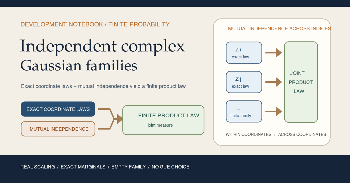
Figure. Exact marginal laws and mutual independence have different jobs. The bundle records both, the finite theorem combines them into a product joint law, and the canonical product space runs the construction in reverse. The empty branch is part of the same product measure API. The diagram neither constructs a matrix ensemble nor contains a proof of a symmetry law.
Why one variable is not enough
A random matrix contains many random coordinates. Even before imposing Hermitian symmetry, one must say how those coordinates coexist on the same outcome space. Knowing the law of each coordinate separately is not enough. Two vectors can share every marginal distribution and still have completely different dependence.
For a finite index type \(\iota\), consider maps
\[ Z_i:\Omega\to\mathbb C, \qquad i\in\iota, \]on a measured outcome space \((\Omega,P)\). The data attached to coordinate \(i\) are
\[ m_i\in\mathbb C, \qquad v_{\mathrm{Re},i},v_{\mathrm{Im},i}\in\mathbb R_{\ge 0}. \]The one-variable module gives the exact law
\[ \Gamma_i = \operatorname{cartesianComplexGaussian} (m_i,v_{\mathrm{Re},i},v_{\mathrm{Im},i}). \]That law already says that the real and imaginary parts of \(Z_i\) are independent Gaussian coordinates. It says nothing about the relation between \(Z_i\) and \(Z_j\) when \(i\ne j\). The new module adds precisely that second layer.
If the family is mutually independent, its function-valued sample map
\[ Z:\Omega\longrightarrow(\iota\to\mathbb C), \qquad Z(\omega)(i)=Z_i(\omega), \]has the product law
\[ \mathcal L_P(Z) = \operatorname{Measure.pi}(i\mapsto\Gamma_i). \]This equality is stronger than a row of marginal statements. It specifies the probability assigned to every measurable event in the finite coordinate space, including events that couple several coordinates.
Lineage, local contribution, and nonclaims
The mathematical ingredients are standard finite-product probability,
implemented against the repository’s pinned
Mathlib 4.32.0 release:
measurable coordinate maps, exact pushforward laws, mutual independence, and
finite product measures. The Lean implementation reuses Mathlib’s HasLaw,
iIndepFun, Measure.pi, measurePreserving_eval, and Gaussian-law APIs
(Mathlib HasLaw,
finite product measures,
independence).
This module’s local contribution is a normalization-explicit interface for the project’s next random-matrix steps:
- every complex coordinate keeps a mean and two nonnegative real variances;
- ordinary measurability is recorded separately from exact law;
- real-imaginary independence inside a coordinate is kept distinct from mutual independence across complex coordinates;
- real coordinatewise scaling preserves the whole bundle with an exact variance formula;
- finite families acquire an exact product joint law and qualitative joint Gaussianity;
- a canonical product sample space realizes the bundle; and
- the empty-index law is named explicitly rather than left to an implicit simplifier.
Not claimed
- No coordinate is called standard without a variance convention.
- No general complex scalar multiplication theorem is stated.
- No matrix is constructed, and no Hermitian support theorem follows here.
- No GUE density, dimension scaling, unitary invariance, eigenvalue law, trace expectation, or large-dimension limit is proved.
- No theorem infers independence between two real families from separate within-family independence assumptions.
- The empty scalar product law does not decide what a zero-dimensional matrix ensemble should mean.
The independence hierarchy
The word “independent” occurs at several levels. Mixing them is the most dangerous conceptual error in this slice.
Level one: inside one complex coordinate
Writing \(Z_i=X_i+iY_i\), the exact Cartesian law says
\[ \mathcal L_P(X_i,Y_i) = \gamma_{(m_i)_{\mathrm{Re}},v_{\mathrm{Re},i}} \otimes \gamma_{(m_i)_{\mathrm{Im}},v_{\mathrm{Im},i}}. \]Thus \(X_i\) and \(Y_i\) are independent. This is already stored in
HasCartesianComplexGaussianLaw.
Level two: across complex coordinates
The family field independent : iIndepFun Z P says that the complex-valued
maps \((Z_i)_{i\in\iota}\) are mutually independent. For a finite family,
every measurable rectangle factors in the expected way. More importantly for
Lean, Mathlib turns that condition plus the exact coordinate laws into an exact
product HasLaw theorem.
Level three: pair vectors before complex assembly
Suppose the raw inputs are real pairs \((X_i,Y_i)\). To map each pair to \(X_i+iY_i\), the constructor needs two kinds of evidence:
- the law of each pair is the product of its requested real Gaussian laws;
- the pair-valued maps \(i\mapsto(X_i,Y_i)\) are mutually independent.
Separate independence of the \(X\)-family and the \(Y\)-family does not imply the second fact. Even adding pairwise independence inside every displayed pair does not generally supply all mixed independence.
A finite-sign example makes the gap visible. Let \(A,B,C\) be independent fair random signs (Rademacher variables). Set
\[ (X_1,Y_1)=(A,C), \qquad (X_2,Y_2)=(B,ABC). \]The two \(X\)-coordinates are independent. The two \(Y\)-coordinates are independent. Each displayed pair also has independent components. Yet the two pair vectors cannot be independent because their four components satisfy the deterministic relation
\[ X_1Y_1X_2Y_2=1. \]This example is not a Gaussian construction and is not part of the Lean file. Its job is structural: it shows why a theorem must request independence of the pair vectors themselves instead of trying to manufacture it from weaker lists of assumptions.
Camp one: exact real scaling
HasCartesianComplexGaussianLaw.real_smul
Before scaling an entire family, the file proves the one-coordinate theorem. If \(Z\) has mean \(m\) and coordinate variances \(v_{\mathrm{Re}}\) and \(v_{\mathrm{Im}}\), then for \(c\in\mathbb R\),
\[ cZ \sim \Gamma^{\mathrm{cart}}_{cm; c^2v_{\mathrm{Re}},c^2v_{\mathrm{Im}}}. \]The checked parameters use an NNReal wrapper around \(c^2\), carrying the
proof sq_nonneg c that the scaled variance remains nonnegative. Negative
scales are allowed. At \(c=0\), both coordinate variances vanish and the law
is the Dirac measure at the origin. The proof uses Mathlib’s exact
real Gaussian scaling API and its treatment of
complex numbers as a real normed space.
The proof exposes rather than hides the coordinate mechanism:
- map both real and imaginary parts through multiplication by \(c\);
- preserve their independence with
IndepFun.compand measurable scaling; - apply the prior constructor
of_indep_re_imto the two scaled real laws; - prove that the reconstructed complex expression equals complex real scalar multiplication by extensionality on real and imaginary parts; and
- rewrite complex multiplication by a coerced real as
c • ZusingComplex.real_smul.
Why only a real scalar? A general complex multiplier \(a+ib\) transforms the coordinate pair by
\[ \begin{pmatrix} \operatorname{Re}((a+ib)Z)\\ \operatorname{Im}((a+ib)Z) \end{pmatrix} = \begin{pmatrix} a&-b\\ b&a \end{pmatrix} \begin{pmatrix} \operatorname{Re}Z\\ \operatorname{Im}Z \end{pmatrix}. \]That rotation-and-scaling can mix the axes and can create nonzero coordinate covariance when the original variances differ. A correct general theorem would need a covariance-aware target law. The current Cartesian interface deliberately proves the operation that preserves its axis-aligned form.
Camp two: the family bundle
IndependentCartesianComplexGaussianFamily
The central structure packages three obligations:
structure IndependentCartesianComplexGaussianFamily
    (Z : ι → Ω → ℂ) (m : ι → ℂ) (vRe vIm : ι → ℝ≥0)
    (P : Measure Ω) : Prop where
  measurable : ∀ i, Measurable (Z i)
  hasLaw : ∀ i, HasCartesianComplexGaussianLaw (Z i) (m i) (vRe i) (vIm i) P
  independent : iIndepFun Z P
The structure is a proposition, not a new random-variable data type. A proof
of it certifies an existing family \(Z\). The family may have any index type;
finiteness appears only for conclusions that use Mathlib’s finite
Measure.pi.
The first field is intentionally ordinary Measurable, not merely
AEMeasurable. An exact HasLaw includes almost-everywhere measurability, but
later constructions often need composable ordinary sample maps. Keeping the
stronger fact as its own field prevents accidental upgrades.
The second field is local distributional data. The third is global dependence data. Neither can replace the other.
IndependentCartesianComplexGaussianFamily.aemeasurable
For each index \(i\), ordinary measurability immediately yields
AEMeasurable (Z i) P. The theorem is a convenience projection with an
important direction: it weakens ordinary measurability to the a.e. form. It
does not travel backward.
IndependentCartesianComplexGaussianFamily.isProbabilityMeasure
The bundle implies IsProbabilityMeasure P through
hZ.independent.isProbabilityMeasure. Mathlib’s iIndepFun includes
normalization of the base measure, so this remains true even if the index type
is empty. There is no need to choose an arbitrary coordinate just to recover
probability normalization.
IndependentCartesianComplexGaussianFamily.real_hasLaw
At coordinate \(i\), the real part has exact law
\[ \operatorname{Re}Z_i \sim \gamma_{\operatorname{Re}m_i,v_{\mathrm{Re},i}}. \]The proof delegates to (hZ.hasLaw i).real_hasLaw. It inherits the exact
one-variable marginal theorem rather than recomputing a pushforward.
IndependentCartesianComplexGaussianFamily.imag_hasLaw
Likewise,
\[ \operatorname{Im}Z_i \sim \gamma_{\operatorname{Im}m_i,v_{\mathrm{Im},i}}. \]The separate theorem matters because the two variance functions need not be equal.
IndependentCartesianComplexGaussianFamily.mean_eq
Every coordinate is integrable and has exact complex expectation
\[ \int_\Omega Z_i(\omega)\,dP(\omega)=m_i. \]The proof is one line through (hZ.hasLaw i).mean_eq. The family layer adds no
new analytic argument; it makes the scalar result uniformly available by
index.
IndependentCartesianComplexGaussianFamily.real_variance_eq
The checked real-coordinate variance is
\[ \operatorname{Var}_P(\operatorname{Re}Z_i) =v_{\mathrm{Re},i}. \]Lean coerces the nonnegative parameter from NNReal to Real on the right.
This is variance, not standard deviation.
IndependentCartesianComplexGaussianFamily.imag_variance_eq
The imaginary-coordinate companion is
\[ \operatorname{Var}_P(\operatorname{Im}Z_i) =v_{\mathrm{Im},i}. \]Together the two declarations preserve the normalization ledger coordinate by coordinate.
IndependentCartesianComplexGaussianFamily.memLp
For every coordinate, every extended nonnegative exponent \(p\ne\infty\)
satisfies MemLp (Z i) p P. This includes every positive finite moment order
and Mathlib’s special \(p=0\) case. At \(p=0\), MemLp records almost-
everywhere strong measurability; it should not be advertised as a zeroth
moment estimate. The theorem makes no \(L^\infty\) claim.
IndependentCartesianComplexGaussianFamily.integrable
Every coordinate is Bochner integrable as a complex-valued function. This is exactly the analytic fact needed to speak about coordinate expectations. It does not yet prove that a matrix-valued assembly, a trace power, or an eigenvalue statistic is integrable. Those require their own finite-dimensional bounds and measurable constructions.
Camp three: construct complex coordinates from independent pair laws
IndependentCartesianComplexGaussianFamily.of_independent_real_pair_laws
The longest theorem is the safest constructor. It begins with real-valued families \(X_i,Y_i\) and asks for:
- ordinary measurability of every pair map \(\omega\mapsto(X_i(\omega),Y_i(\omega))\);
- an exact product Gaussian law for every pair; and
- mutual independence of the pair-valued maps across \(i\).
Its output is the complex family
\[ Z_i=X_i+iY_i \]with means \(m_i\), variance functions \(v_{\mathrm{Re}}\) and \(v_{\mathrm{Im}}\), and the full family bundle.
The proof fills the three structure fields in the same order as the definition.
For measurability, it composes each measurable pair map with the measurable pairing function \((x,y)\mapsto x+iy\).
For the exact law, it uses Complex.equivRealProdCLM.symm as a HasLaw map
from the real product measure to cartesianComplexGaussian. It composes that
law with hPairLaw i, then closes the pointwise expression mismatch with
HasLaw.congr and the formula for the equivalence.
For mutual independence, it applies hPairs.comp to the same measurable
pairing map at every coordinate. Measurable coordinatewise maps preserve
mutual independence.
Camp four: scale a whole family
IndependentCartesianComplexGaussianFamily.scale
Given real factors \(c_i\), define
\[ Z_i'=c_i Z_i. \]The output bundle has mean and variances
\[ m_i'=c_i m_i, \qquad v_{\mathrm{Re},i}'=c_i^2v_{\mathrm{Re},i}, \qquad v_{\mathrm{Im},i}'=c_i^2v_{\mathrm{Im},i}. \]The proof again follows the three bundle fields:
Measurable.const_smulproves ordinary measurability;HasCartesianComplexGaussianLaw.real_smulproves each exact law; andiIndepFun.comppreserves mutual independence under the measurable map \(z\mapsto c_i z\).
Each coordinate may use a different real factor. Zero factors are allowed and collapse those coordinates to deterministic zero variables. Negative factors reflect the corresponding complex coordinate through the origin. Both cases remain inside the same theorem because the variance formula uses \(c_i^2\).
The theorem does not choose \(c_i\) as a function of a matrix dimension. Writing a generic coordinatewise scaling operation first keeps later choices such as \(1/\sqrt n\) visible in the ensemble constructor where their meaning can be audited.
High camp: the finite joint law
The next two declarations add [Fintype ι]. This is the point where an
arbitrary indexed family becomes a finite random vector.
IndependentCartesianComplexGaussianFamily.jointHasLaw
The exact statement is
\[ \operatorname{HasLaw} \left( \omega\mapsto(i\mapsto Z_i(\omega)), \operatorname{Measure.pi}(i\mapsto\Gamma_i), P \right). \]The proof is the compact call
hZ.independent.hasLaw_pi hZ.hasLaw
That line is short because the bundle was designed to match Mathlib’s theorem.
hZ.independent supplies the factorization structure; hZ.hasLaw supplies
every exact marginal. The result includes a.e. measurability of the whole
function-valued sample map and equality of its pushforward with the finite
product measure.
IndependentCartesianComplexGaussianFamily.jointHasGaussianLaw
After forgetting the explicit means and variance pairs, the full vector is Gaussian in Mathlib’s qualitative sense:
\[ \operatorname{HasGaussianLaw} (\omega\mapsto(i\mapsto Z_i(\omega)))\ P. \]The proof uses mutual independence together with the qualitative Gaussian law of every coordinate through Mathlib’s Gaussian independence API. The result concerns the real Banach-space structure on the finite function space \(\iota\to\mathbb C\). It does not assert complex circularity, equal covariance, or a matrix symmetry class.
The exact jointHasLaw theorem should be preferred whenever normalization
matters. The qualitative theorem is useful for generic Gaussian closure and
integrability APIs, but it intentionally forgets the parameter ledger.
Summit camp: the canonical product sample space
The family bundle can certify random variables on any outcome space. The final six declarations also provide a concrete outcome space when no other model is needed.
cartesianComplexGaussianProductMeasure
On the coordinate space \(\iota\to\mathbb C\), define
\[ P_{\mathrm{prod}} = \operatorname{Measure.pi}(i\mapsto\Gamma_i). \]This is the canonical finite product of the requested coordinate laws. Its sample points are complete complex coordinate vectors. No simulation or choice of random-number generator is involved; this is a mathematical probability space.
instIsProbabilityMeasureCartesianComplexGaussianProduct
Every factor \(\Gamma_i\) is already a probability measure. Mathlib’s product
instance therefore proves that cartesianComplexGaussianProductMeasure is a
probability measure. The implementation unfolds the project definition and
lets typeclass inference assemble the result.
cartesianComplexGaussianProductMeasure_hasLaw_eval
Fix an index \(i\). Evaluation
\[ \operatorname{ev}_i:(\iota\to\mathbb C)\to\mathbb C, \qquad \operatorname{ev}_i(z)=z_i, \]has exactly the law \(\Gamma_i\) under \(P_{\mathrm{prod}}\). The proof uses
Mathlib’s measurePreserving_eval and extracts its HasLaw consequence.
This is the formal marginal property of the product construction.
cartesianComplexGaussianProductMeasure_iIndepFun
The evaluation maps are mutually independent under the canonical product
measure. iIndepFun_pi supplies the theorem after receiving the a.e.
measurability of the identity map at every coordinate. This is the formal
factorization property of the same construction.
The evaluation-law theorem and the independence theorem are separate because they answer different questions. One names each coordinate distribution. The other names their dependence.
cartesianComplexGaussianProductMeasure_independentFamily
The previous facts assemble into the central bundle:
IndependentCartesianComplexGaussianFamily
  (fun i (z : ι → ℂ) ↦ z i) m vRe vIm
  (cartesianComplexGaussianProductMeasure m vRe vIm)
Ordinary measurability comes from measurable_pi_apply. Exact laws come from
the evaluation theorem. Mutual independence comes from iIndepFun_pi. This
declaration is a reusable existence witness for later finite coordinate
constructions.
cartesianComplexGaussianProductMeasure_eq_dirac_of_isEmpty
If \(\iota\) is empty, there is exactly one function \(\iota\to\mathbb C\): the empty function. The finite product measure becomes
\[ P_{\mathrm{prod}} = \delta_{\lambda i,\operatorname{isEmptyElim}(i)}. \]The proof unfolds the project definition and applies Measure.pi_of_empty.
This is not an error case. It is the identity object for finite products,
expressed as a normalized law on a one-point function space.
The theorem deliberately says nothing about matrices of dimension zero. A future matrix constructor may use an index type derived from a dimension and may contain factors such as \(1/n\). Whether such a constructor accepts \(n=0\) is a separate interface decision.
The entire Lean file as a declaration map
| Declaration | What it checks | Main proof engine |
|---|---|---|
HasCartesianComplexGaussianLaw.real_smul | A real scalar scales the mean and both variances exactly | Real marginal scaling, IndepFun.comp, complex extensionality |
IndependentCartesianComplexGaussianFamily | Measurability, exact laws, and mutual independence in one proposition | Three-field structure |
.aemeasurable | Every coordinate is a.e. measurable | Measurable.aemeasurable |
.isProbabilityMeasure | The common base measure is normalized | iIndepFun.isProbabilityMeasure |
.real_hasLaw | Exact real-part Gaussian law at index \(i\) | One-coordinate marginal theorem |
.imag_hasLaw | Exact imaginary-part Gaussian law at index \(i\) | One-coordinate marginal theorem |
.mean_eq | Exact complex coordinate mean | One-coordinate expectation theorem |
.real_variance_eq | Exact real-coordinate variance | Exact real Gaussian variance |
.imag_variance_eq | Exact imaginary-coordinate variance | Exact real Gaussian variance |
.memLp | Coordinate MemLp for every \(p\ne\infty\) | Qualitative Gaussian MemLp |
.integrable | Complex coordinate integrability | Qualitative Gaussian integrability |
.of_independent_real_pair_laws | Pair-valued real inputs become an independent complex family | HasLaw.comp, HasLaw.congr, iIndepFun.comp |
.scale | Coordinatewise real scaling preserves the bundle | Scalar real_smul plus measurable independence transport |
.jointHasLaw | Exact finite product joint law | iIndepFun.hasLaw_pi |
.jointHasGaussianLaw | Qualitative joint Gaussianity | iIndepFun.hasGaussianLaw |
cartesianComplexGaussianProductMeasure | Canonical product law on \(\iota\to\mathbb C\) | Measure.pi |
instIsProbabilityMeasureCartesianComplexGaussianProduct | Product normalization | Probability-measure typeclass inference |
cartesianComplexGaussianProductMeasure_hasLaw_eval | Exact evaluation marginal | measurePreserving_eval |
cartesianComplexGaussianProductMeasure_iIndepFun | Mutual independence of evaluations | iIndepFun_pi |
cartesianComplexGaussianProductMeasure_independentFamily | Canonical evaluations satisfy the family bundle | Structure assembly |
cartesianComplexGaussianProductMeasure_eq_dirac_of_isEmpty | Empty product is the Dirac law at the empty function | Measure.pi_of_empty |
Twenty-one public declarations form one dependency chain. None is an isolated helper disguised as a result: each either preserves exact normalization data, bridges a dependence layer, or exposes a reusable canonical construction.
Proof architecture: four reusable moves
1. Transport laws through measurable maps
HasLaw.comp is the principal law-transport lemma used here. The
pair constructor maps \((X_i,Y_i)\) through the real-linear identification
with \(\mathbb C\). Exactness is preserved because both the input law and the
map’s pushforward law are named.
2. Preserve independence coordinatewise
Both scalar scaling and pair-to-complex assembly use iIndepFun.comp.
Measurable functions applied separately to mutually independent coordinates
remain mutually independent. Its application here requires input independence
at the correct block level.
3. Match the bundle to the upstream finite-product theorem
The fields hasLaw and independent are precisely the inputs to
iIndepFun.hasLaw_pi. As a result, the global law theorem is one line because
the interface records all of its hypotheses.
4. Prove the canonical realization theorem by evaluation
Measure.pi comes with two complementary APIs: evaluation is
measure-preserving onto each factor, and the evaluation maps are mutually
independent. Those facts reproduce all three fields of the project bundle on
the product sample space.
Exact commands: compile, cover, and preview
Load elan in a fresh shell:
source "$HOME/.elan/env"
Compile the changed module with warnings promoted to errors:
cd formalization
lake env lean -DwarningAsError=true NonlinearDynamics/Random/ComplexGaussianFamilies.lean
Compile the Random aggregator and root import graph as additional checks:
cd formalization
lake env lean -DwarningAsError=true NonlinearDynamics/Random.lean
lake env lean -DwarningAsError=true NonlinearDynamics.lean
From the repository root, validate the proof-to-prose mapping and Hugo site:
python3 scripts/check_lean_notebook_coverage.py
make site-check
Regenerate or verify this page’s social card from any working directory:
site/content/development-notebook/2026/07/independent-complex-gaussian-families/generate-card.sh
site/content/development-notebook/2026/07/independent-complex-gaussian-families/generate-card.sh --verify
Starting from the repository root, build the complete formalization and check the public teaching content:
cd formalization
lake build

cd ..
make content-hygiene
make site-check
Preview all drafts locally on port 1333:
make blog-serve
Worked finite family
Take a three-coordinate index type and choose
\[ m=(m_0,m_1,m_2), \qquad v_{\mathrm{Re}}=(r_0,r_1,r_2), \qquad v_{\mathrm{Im}}=(s_0,s_1,s_2). \]No equality among the \(r_i\) or \(s_i\) is required. A proof of
IndependentCartesianComplexGaussianFamily Z m vRe vIm P gives, all at once:
- \(Z_0,Z_1,Z_2\) are ordinarily measurable;
- each \(Z_i\) has its exact two-variance Cartesian law;
- the three complex variables are mutually independent;
- their means and real-imaginary variance pairs can be recovered by index;
- each coordinate is integrable and has every finite
MemLpexponent; and - the vector \(\omega\mapsto(Z_0(\omega),Z_1(\omega),Z_2(\omega))\) has exactly the product of the three stated laws.
Now choose real scales \(c_0,c_1,c_2\). The .scale theorem returns the same
bundle for \((c_0Z_0,c_1Z_1,c_2Z_2)\), with no manual re-proof of independence.
This is the algebraic shape needed when future matrix coordinates receive
different deterministic normalizations.
The example remains deliberately generic. It does not say that three coordinates are enough for a particular matrix, nor that equal component variances would establish unitary invariance.
Edge-case register
| Case | Checked behavior | Boundary |
|---|---|---|
| \(c_i=0\) | Scaled coordinate is deterministic zero with both variances zero | Other coordinates and their laws remain present |
| \(c_i\lt 0\) | Mean is reflected and both variances scale by \(c_i^2\) | No sign enters a variance |
| Exactly one of \(v_{\mathrm{Re},i}\), \(v_{\mathrm{Im},i}\) is zero | Exact Cartesian law remains valid | Line-supported geometry has no separate family theorem |
| Both variances zero | Coordinate law is Dirac at its mean through the one-variable layer | The family may contain deterministic coordinates |
| Empty \(\iota\) | Canonical product law is Dirac at the unique empty function | This does not choose a zero-dimensional matrix policy |
| Infinite \(\iota\) | The family structure itself is available | jointHasLaw and the canonical Measure.pi in this file require Fintype |
\(p=0\) in memLp | A.e. strong measurability is retained | This is not a moment estimate |
| \(p=\infty\) | No theorem is stated | Nondegenerate Gaussians are not essentially bounded |
| General complex scaling | Not formalized | Axis mixing needs covariance-aware bookkeeping |
Failure modes this interface prevents
A list of marginals masquerading as a joint law
Statements of the form \(Z_i\sim\Gamma_i\) do not determine
\(\mathcal L((Z_i)_i)\). The explicit iIndepFun field and jointHasLaw
theorem close that gap.
Independence at the wrong granularity
Separate real-family and imaginary-family independence can miss cross-family dependencies. The pair constructor requires mutual independence of the pair vectors it actually transforms.
Hiding a factor of two
Every coordinate retains both \(v_{\mathrm{Re},i}\) and \(v_{\mathrm{Im},i}\). A future symmetric choice still has to say whether each component has variance \(1/2\), \(1\), or a dimension-dependent scale.
Treating HasLaw as ordinary measurability
HasLaw supplies a.e. measurability. The bundle records ordinary
measurability separately, and its .aemeasurable theorem only weakens that
fact in the valid direction.
Using real scaling as a hidden GUE normalization
The .scale theorem accepts an arbitrary function \(c_i\). It proves how
laws transform but endorses no specific matrix dimension, variance, or trace
scale.
Calling a product vector a Hermitian matrix
An element of \(\iota\to\mathbb C\) is a coordinate vector. Hermitian matrix assembly must still place real variables on the diagonal, complex variables above the diagonal, conjugates below it, and prove the resulting law’s properties.
Reading joint Gaussianity as circularity
jointHasGaussianLaw uses Mathlib’s real Banach-space notion. It does not
state equal component variances, zero pseudocovariance, circular symmetry, or
unitary invariance.
Exercises
- For a singleton index type, show on paper that
jointHasLawreduces to the one coordinate law after identifying singleton functions with \(\mathbb C\). Which equivalence would Lean need? - Set one scale factor to zero and explain which three fields of the family
bundle the
.scaleproof must re-establish. - Give two complex random variables with the same Cartesian marginals but different joint laws. Which field distinguishes them?
- In the finite-sign counterexample above, verify each pairwise independence statement and then use the deterministic four-variable product to reject block independence.
- Explain why
hPairLawin the constructor carries more information than separate laws for \(X_i\) and \(Y_i\). - Derive the covariance of the transformed real and imaginary parts after multiplying an anisotropic centered Cartesian law by \(a+ib\). Identify the condition under which the transformed coordinates remain uncorrelated.
- Compare the exact theorem
jointHasLawwith the qualitative theoremjointHasGaussianLaw. List the normalization data forgotten by the latter. - For an empty index type, explain why the function space contains one point even though there are no coordinates to evaluate.
- Sketch an index type for the strict upper triangle of an \(n\times n\) matrix. Which additional real family is needed for the diagonal?
- Write a normalization ledger for a possible Wigner-scaled Hermitian matrix, but leave every choice labeled as a proposal rather than a theorem.
The next ridge: independent entries are not yet GUE
This module supplies the probability engine for independent complex coordinates. A finite Hermitian Gaussian matrix requires more structure.
One natural entrywise route uses:
- a real Gaussian family for diagonal entries;
- a Cartesian complex Gaussian family indexed by strict upper-triangular pairs;
- a deterministic matrix assembly that mirrors upper-triangular entries by complex conjugation; and
- a proof that the assembled map is measurable and Hermitian.
Even that construction is not yet GUE. A normalization ledger must specify at least the diagonal variance, off-diagonal real variance, off-diagonal imaginary variance, matrix dimension dependence, density exponent, spectral scale, trace convention, and behavior at dimension zero. Different choices produce different laws.
The hardest symmetry step remains beyond independent coordinates. An entrywise construction makes independence transparent, while unitary invariance is often cleaner from an isotropic Gaussian law on the real vector space of Hermitian matrices. If both representations are used, their equality must be proved. The project will not treat a familiar name as a substitute for that theorem. Dyson’s original symmetry-class analysis supplies historical motivation for the unitary class, not the missing project theorem (Dyson, 1962).
After the GUE law itself is checked, integrability of individual entries will help establish integrability of finite matrix observables. It still does not automatically prove exact expected trace moments. Matrix power, trace, linearity, finite sums, and the ensemble’s dependence structure must all enter those proofs.
Summit register
The checked milestone now contains:
- one-variable real scaling with exact two-variance bookkeeping;
- a measurable mutually independent Cartesian complex Gaussian family bundle;
- exact real and imaginary marginal laws at every coordinate;
- exact coordinate means and component variances;
- coordinate
MemLpand integrability consequences; - a block-level constructor from independent real pair laws;
- coordinatewise real scaling that preserves the bundle;
- an exact finite product joint law;
- qualitative joint Gaussianity;
- a canonical product probability measure and its evaluation family; and
- an explicit empty-index Dirac theorem.
The next milestone must add a matrix representation and a fully approved normalization ledger before using the name GUE. The current result is exactly the family layer needed for that ascent, and no more.
References
The technical references below were checked against the official Mathlib documentation and the exact source revision pinned by this repository. The historical random-matrix reference is linked to its original journal record.
Mathlib contributors.
Mathlib 4.32.0 release,
commit
81a5d257c8e410db227a6665ed08f64fea08e997.
This is the exact dependency revision recorded by the project.
Mathlib contributors. Law of a random variable, with pinned source. This is the primary API source for exact pushforward laws, composition, congruence, finite product laws, and qualitative Gaussian consequences.
Mathlib contributors.
Finite product measures,
with
pinned source.
This is the primary API source for Measure.pi, evaluation marginals,
probability normalization, and the empty-product theorem.
Mathlib contributors.
Independence of families,
with
pinned source.
This is the primary API source for IndepFun, iIndepFun, preservation under
measurable coordinatewise maps, and independence of product evaluations.
Mathlib contributors. Real Gaussian distributions, with pinned source. This is the primary API source for exact real Gaussian laws, means, variances, real scaling, and the zero-variance boundary.
Mathlib contributors. Gaussian independence, with pinned source. This is the primary API source for qualitative joint Gaussianity of finite independent Gaussian coordinates.
Mathlib contributors. Complex numbers as a real normed space, with pinned source. This is the primary API source for real scalar multiplication and the continuous real-linear equivalence between \(\mathbb C\) and \(\mathbb R\times\mathbb R\).
Freeman J. Dyson. Statistical Theory of the Energy Levels of Complex Systems. I, Journal of Mathematical Physics 3, 140-156, 1962. This original article is cited only for the historical symmetry-class motivation. It does not supply a GUE theorem for the current coordinate-family module.