This is the proof-to-prose companion for
formalization/NonlinearDynamics/Random/RandomCocycles/Discrete.lean.
It covers all sixteen public declarations in source order. There are no private
declarations in the module.
The immediate predecessor, Measurable Finite Matrix Products in Lean, separated pointwise products, ordinary measurability, and proof-carrying pushforward laws. RMT-13 consumes its first two floors. Existing glossary foundations include one-sided discrete matrix cocycle , finite random-matrix product , forward matrix product , random matrix , and measurable space . The parallel textbook treatment is Generator-Presented One-Sided Discrete Matrix Cocycles.
Choose a route up
| Route | Begin | Destination |
|---|---|---|
| First encounter | One generator creates a time sequence | See how a base orbit turns one observation rule into changing matrices |
| Convention route | The first four cocycle values | Audit natural iterates and newest-factor-left multiplication |
| Algebra route | The exact later-block-left identity | Split time without reversing the base shift or matrix order |
| Measurability route | Measurability climbs through the orbit | Compose the generator with base iterates and reuse finite-product closure |
| Bundling route | What the cocycle structure actually stores | Separate stored generator data from derived cocycle values |
| Measure route | Every base iterate preserves the measure | Read MeasurePreserving without assuming probability or ergodicity |
| Boundary route | Empty matrix dimension remains valid | Understand why no Nonempty hypothesis appears |
| Lean route | The complete declaration map | Inspect all sixteen declarations in source order |
| Integrity route | Strict nonclaims | Separate finite cocycle algebra from stochastic and asymptotic theory |
Learning objectives
By the summit, a reader should be able to:
- distinguish a base map from a matrix generator;
- state Mathlib’s natural-number iterate convention at times zero and one;
- explain how one generator produces a time-indexed orbit matrix sequence;
- expand the first four finite cocycle values without reversing a factor;
- explain why the newest observation is written on the left;
- state the exact cocycle identity at times \(m\) and \(k\);
- explain why the later block is evaluated at \(T^m\omega\);
- audit the identity at both zero-length boundaries;
- distinguish the assumption-free orbit observation from the finite-semiring product floor used by declarations two through six;
- prove measurability of each observed factor by composition;
- prove measurability of every finite cocycle value by the RMT-12 prefix theorem;
- list all four fields stored by
DiscreteMatrixCocycle; - explain why the structure is generator presented rather than an arbitrary cocycle-law bundle;
- distinguish measure preservation from probability normalization;
- distinguish measure preservation from ergodicity, mixing, and invertibility;
- derive the structure’s zero, one, successor, and addition laws;
- derive ordinary measurability of every bundled value;
- explain why every base iterate preserves the same measure;
- explain why the matrix index type is irrelevant to the base-iterate theorem;
- interpret the complete interface in empty matrix dimension; and
- identify every hypothesis still missing before logarithmic growth or a multiplicative ergodic theorem.
Lineage, contribution, and boundary
Matrix cocycles are standard in random dynamical systems, derivative dynamics, and products of random matrices. Classical asymptotic work adds measure-theory and integrability hypotheses to study growth, with Furstenberg and Kesten’s random-product paper as one early landmark (Furstenberg and Kesten, 1960). This chapter does not claim to invent cocycles or to formalize that asymptotic theorem.
The local contribution is a small generator-presented Lean interface whose time and multiplication conventions are frozen and testable. It derives the cocycle identity directly from base iteration, separates algebra from measurability, and packages precisely a measure-preserving base plus a measurable complex matrix generator. The result is finite-time infrastructure, not an ergodic conclusion.
One generator creates a time sequence
Begin with two functions on the same environment space \(\Omega\):
\[ T:\Omega\to\Omega, \qquad A:\Omega\to\operatorname{Matrix}(\iota,\iota,\mathbb K). \]The base map \(T\) advances the environment. The generator \(A\) reads a matrix from whichever environment point it receives. Starting from \(\omega\), the forward base orbit is
\[ \omega,\quad T\omega,\quad T^2\omega,\quad T^3\omega,\quad\ldots \]and the corresponding matrix observations are
\[ A(\omega),\quad A(T\omega),\quad A(T^2\omega),\quad A(T^3\omega),\quad\ldots \]This is different from supplying an arbitrary time-indexed sequence \(A_0,A_1,A_2,\ldots\). Every time slice is generated by the same observation rule after advancing the same base dynamics.
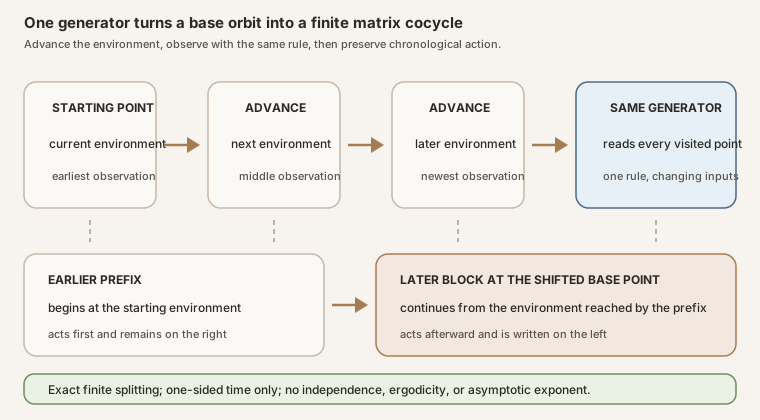
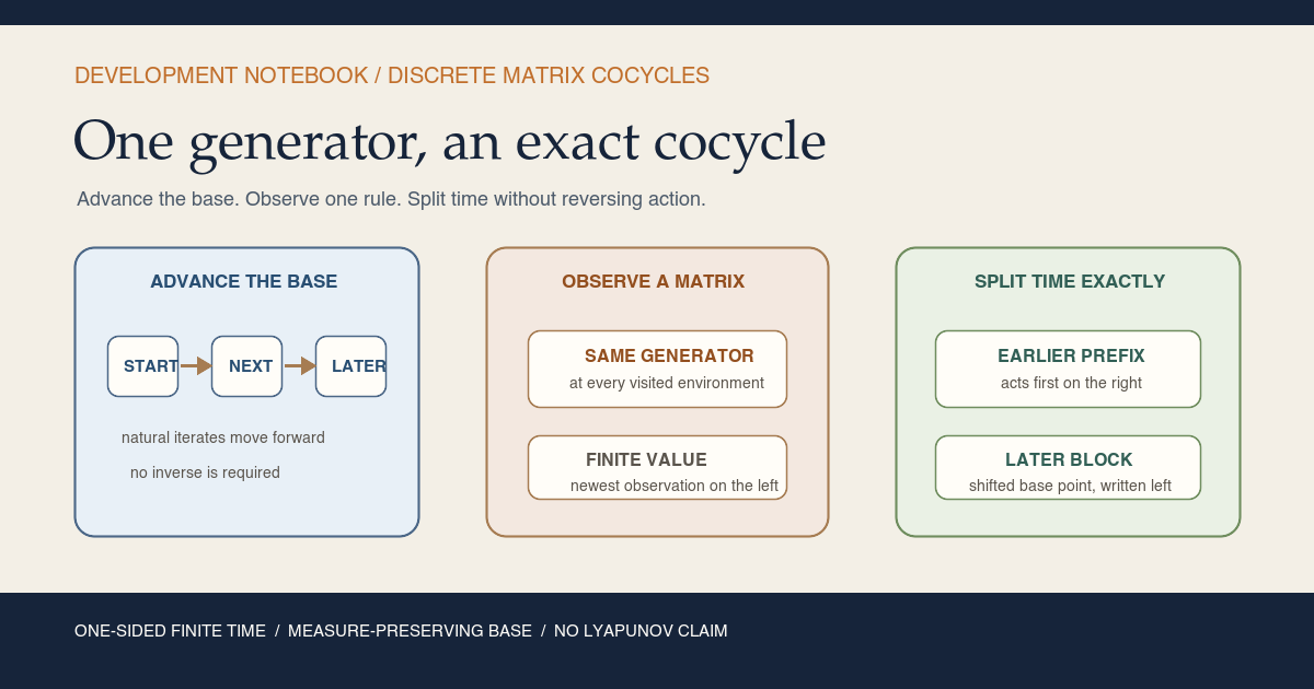
Figure: the base advances the environment, while one reusable generator observes a matrix at each visited point. The finite value multiplies later observations on the left, so a time split evaluates the later block at the shifted base point. The plate asserts no inverse time, ergodicity, independence, or asymptotic exponent.
Declaration 1: orbitMatrixSequence
The source encodes the observation sequence as
def orbitMatrixSequence (T : Ω → Ω)
    (A : RandomMatrix Ω ι ι 𝕜) :
    ℕ → RandomMatrix Ω ι ι 𝕜 :=
  fun j ω => A (T^[j] ω)
Mathlib writes the \(j\)-fold iterate as T^[j]. Its base cases
are
The output at each \(j\) is still a matrix-valued function on \(\Omega\). No measure or measurability proof is involved in this definition.
Declaration 2: cocycleProduct
The second definition hands that sequence to RMT-12’s pointwise finite product:
def cocycleProduct (T : Ω → Ω)
    (A : RandomMatrix Ω ι ι 𝕜) (k : ℕ) :
    RandomMatrix Ω ι ι 𝕜 :=
  MatrixProducts.sampleForwardProduct (orbitMatrixSequence T A) k
Write its value as \(\Phi_{T,A}(k,\omega)\). Then
\[ \Phi_{T,A}(k,\omega) =A(T^{k-1}\omega)\cdots A(T\omega)A(\omega). \]The definition does not store a separate sequence of matrices. It regenerates each factor from \(T\), \(A\), the time index, and the initial environment.
The first four cocycle values
Unfolding the definitions gives
\[ \begin{aligned} \Phi(0,\omega) &{}=I,\\ \Phi(1,\omega) &{}=A(\omega),\\ \Phi(2,\omega) &{}=A(T\omega)A(\omega),\\ \Phi(3,\omega) &{}=A(T^2\omega)A(T\omega)A(\omega). \end{aligned} \]The orbit moves forward from left to right in the list of observations. Matrix action is read from right to left, so the earliest observation sits nearest a column vector and the newest observation is written on the left.
Declaration 3: zero time
cocycleProduct_zero says the time-zero value is the constant
identity map. The proof is rfl because both the orbit sequence and
sample-product conventions have identity at the empty horizon.
Declaration 4: one more observation
cocycleProduct_succ exposes the recursion
The factor at the newly visited base point is prepended. This theorem is also
definitional equality and marked @[simp].
Declaration 5: one step
cocycleProduct_one proves equality of matrix-valued functions:
At one step, the iterate has exponent zero, so the generator is evaluated at
the original environment. The Lean proof uses function extensionality and
simplification of cocycleProduct and
orbitMatrixSequence.
The exact later-block-left identity
Declaration 6, cocycleProduct_add, is the algebraic summit of the
module. Split a total horizon after \(m\) steps, then run for another \(k\)
steps. The theorem is
The earlier block \(\Phi(m,\omega)\) acts first and remains on the right. The later block begins from the environment reached after those \(m\) steps, so it is \(\Phi(k,T^m\omega)\), and it acts afterward from the left.
For \(m=2\) and \(k=3\), the equality expands to
\[ \begin{aligned} &A(T^4\omega)A(T^3\omega)A(T^2\omega) A(T\omega)A(\omega)\\ &\qquad{}= \bigl(A(T^4\omega)A(T^3\omega)A(T^2\omega)\bigr) \bigl(A(T\omega)A(\omega)\bigr). \end{aligned} \]This concrete audit checks both moving pieces. The shifted later block starts at \(T^2\omega\), and that entire block is on the left.
Both boundary cases
If \(k=0\), the later block is the identity at \(T^m\omega\):
\[ \Phi(m+0,\omega)=I\Phi(m,\omega). \]If \(m=0\), the base shift is the identity and the earlier block is the identity matrix:
\[ \Phi(0+k,\omega)=\Phi(k,\omega)I. \]Neither boundary needs a separate convention.
The proof architecture
The Lean theorem is pointwise in \(\omega\) and inducts on the later length \(k\). At zero, simplification closes the identity. At a successor, the proof unfolds both successor products and uses the induction hypothesis. The only nontrivial base-orbit bookkeeping is
\[ T^{m+k}\omega=T^k(T^m\omega). \]Mathlib’s Function.iterate_add_apply presents the iterate sum in
one order. The proof first commutes the natural-number addition indices, then
applies that theorem. Finally, matrix associativity aligns the newly prepended
factor with the product of the later and earlier blocks.
No matrix factors commute. The use of Nat.add_comm rearranges time
indices in an iterate identity, not matrix multiplication.
The algebraic assumption floor
The first declaration, orbitMatrixSequence, uses no typeclass
assumption at all. It only composes the generator with a natural iterate of the
base map; at this point a matrix is an indexed function of two
coordinates.
Declarations two through six add
[Fintype ι] [DecidableEq ι] [Semiring 𝕜]. The finite coordinate
type and decidable equality support square matrix identity and multiplication.
The scalar semiring supplies addition, multiplication, and one.
There is no measurable space on \(\Omega\), no topology, no norm, no field division, and no measure. The base map need not be injective, surjective, continuous, or invertible. At this floor, it is only a function used to generate a forward orbit.
The separation matters. The cocycle identity is a consequence of function iteration and associativity. It should not inherit probability or analytic hypotheses merely because later applications will use them.
Measurability climbs through the orbit
The second section adds [MeasurableSpace Ω] and fixes the matrix
scalars to \(\mathbb C\). Its two unbundled theorems build measurability in the
same order as the definitions.
Declaration 7: every orbit observation is measurable
measurable_orbitMatrixSequence assumes ordinary measurability of
the base \(T\) and generator \(A\). For every natural \(j\), it proves
is measurable. The proof is a one-line composition:
hA.comp (hT.iterate j)
Mathlib proves that every finite iterate of a measurable self-map is measurable. Composing the measurable generator with that iterate gives the observed factor.
The theorem explicitly omits [Fintype ι] and
[DecidableEq ι]. No matrices are multiplied here. It only composes
functions into the already equipped matrix measurable space.
Declaration 8: every finite product is measurable
measurable_cocycleProduct restores the shared finite-matrix
assumptions and proves measurability of \(\Phi(k,\cdot)\) for every \(k\).
It calls RMT-12’s measurable_sampleForwardProduct on
orbitMatrixSequence T A.
That imported theorem assumes measurability only for factors with \(j\lt k\). RMT-13 can supply
each one with measurable_orbitMatrixSequence. In fact, the base and
generator hypotheses prove every orbit factor measurable, so the finite prefix
condition is discharged uniformly.
The theorem remains measure free. Ordinary measurability is a property of the maps and measurable spaces. No source measure, probability normalization, or almost-everywhere qualification is needed.
Why complex matrices appear only now
The pointwise cocycle works over an arbitrary semiring. The measurable product reuses the project’s checked entrywise multiplication closure for complex matrices. A more general scalar theorem may be possible under suitable measurable algebra hypotheses, but RMT-13 states only the interface compiled against the current project library.
What the cocycle structure actually stores
Declaration 9 introduces
DiscreteMatrixCocycle. For a raw measure \(\mu\) on \(\Omega\),
the structure stores four fields:
| Field | Type-level job | Mathematical meaning |
|---|---|---|
base | Ω → Ω | Advances the environment by one discrete step |
generator | RandomMatrix Ω ι ι ℂ | Reads the one-step matrix at an environment point |
base_preserving | MeasurePreserving base μ μ | Proves the base is measurable and pushes \(\mu\) to itself |
measurable_generator | Measurable generator | Gives ordinary regularity of the matrix observation |
The structure does not store a separate value for every time and then demand a
cocycle axiom. It stores the smaller generator presentation. The finite values
and their identity law are derived from base and
generator.
This choice prevents incoherent data. An arbitrary family \(\Psi(k,\omega)\) could fail at time zero, multiply in the wrong order, or violate the time split. A generator-presented value satisfies those facts by construction and proof.
Measure preserving is two facts, not a slogan
Mathlib’s MeasurePreserving T μ μ is a proposition with two
components (official documentation):
- \(T\) is measurable; and
Measure.map T μ = μ.
The second component says the base redistributes \(\mu\) without changing the measure. It does not say that \(\mu\) has total mass one. The zero measure, an infinite invariant measure, or a finite nonnormalized invariant measure can all fit the type when the map and equality are appropriate.
Measure preservation also does not mean ergodicity. An invariant measurable set may still have intermediate mass. It does not mean mixing. It does not mean the base is invertible. The structure deliberately records only the two facts in Mathlib’s predicate.
Derived values inherit the cocycle interface
Inside the DiscreteMatrixCocycle namespace, the remaining seven
declarations turn the stored fields into a usable public API.
Declaration 10: value
The finite value is the unbundled cocycle product generated by the stored base and generator:
def value (C : DiscreteMatrixCocycle (ι := ι) μ) (k : ℕ) :
    RandomMatrix Ω ι ι ℂ :=
  cocycleProduct C.base C.generator k
The name value emphasizes that this is the matrix-valued map at one
finite time. It is not a pushforward law, norm, logarithm, or expectation. For
each \(\omega\), C.value k ω is one concrete matrix.
Declaration 11: value_zero
The bundled time-zero value is the constant identity map:
\[ C.\operatorname{value}(0,\omega)=I. \]The theorem is rfl and marked @[simp]. The structure
stores no separate identity axiom because the generator presentation already
forces it.
Declaration 12: value_one
At one step, the value equals the stored generator:
\[ C.\operatorname{value}(1,\cdot)=C.\operatorname{generator}. \]The proof delegates to cocycleProduct_one. This theorem is the
bridge between the abstract word “generator” and its exact operational role:
it is the one-step cocycle value at the current environment.
Declaration 13: value_succ
The bundled successor recursion is
\[ C.\operatorname{value}(k+1,\omega) =C.\operatorname{generator}(C.\operatorname{base}^k\omega) C.\operatorname{value}(k,\omega). \]It is definitional equality. The newest generator observation appears on the
left, exactly as in the unbundled product. Marking the theorem
@[simp] makes finite-horizon reductions discoverable to later
proofs.
Declaration 14: value_add
The bundled cocycle identity is
\[ C.\operatorname{value}(m+k,\omega) =C.\operatorname{value}(k,C.\operatorname{base}^m\omega) C.\operatorname{value}(m,\omega). \]Its proof is exactly cocycleProduct_add specialized to the stored
base and generator. The structure does not make the identity stronger. It
packages the data needed to reuse it without passing four arguments manually.
Declaration 15: measurable_value
Every finite bundled value is ordinarily measurable:
\[ \operatorname{Measurable}\bigl(C.\operatorname{value}(k,\cdot)\bigr). \]The proof calls measurable_cocycleProduct. Its base measurability
comes from C.base_preserving.measurable, while generator
measurability comes from the field C.measurable_generator.
Notice what is reused. The structure does not store both
Measurable C.base and MeasurePreserving C.base μ μ.
The latter already contains the former, so the theorem projects it instead of
duplicating evidence.
measurable_value is the bridge needed to define a proof-carrying
pushforward law of a cocycle value in a later file. RMT-13 itself stops before
naming such a law.
Every base iterate preserves the measure
Declaration 16, base_iterate_preserving, proves
for every natural \(k\). It delegates to Mathlib’s
MeasurePreserving.iterate, which proves the statement by repeated
composition and uses the identity map at zero.
At \(k=0\), the base iterate is the identity and preserves \(\mu\) by the identity pushforward law. At \(k+1\), composition of the already preserving \(k\)-fold iterate with the preserving base remains measure preserving. Both measurability and the pushforward equality travel through composition.
The theorem explicitly omits [Fintype ι] and
[DecidableEq ι]. Although it is a method on a matrix-cocycle
structure, its conclusion talks only about the base and the measure. Matrix
dimension, entries, and multiplication are irrelevant to the proof.
What this theorem permits and what it does not supply
The iterate theorem establishes that the environment distribution is invariant under every finite time advance. It does not prove that time averages converge. It does not prove invariant events are trivial. It does not prove decorrelation. Those are ergodic or mixing conclusions requiring separate hypotheses and theorems.
Nor does the theorem say the generator observations are independent. In fact, they are all deterministic functions of one initial \(\omega\). Measure preservation can make their one-time distributions compatible across shifts, but dependence between times remains entirely open, and RMT-13 exports no distributional theorem about them.
Empty matrix dimension remains valid
No declaration assumes [Nonempty ι]. If \(\iota\) is empty, the
square matrix type has one element because there are no entries at which
matrices can differ. Its identity, zero, and every product presentation are
extensionally the same unique matrix.
The orbit sequence still exists. The cocycle product still has a time-zero identity and satisfies the successor and addition equations. The unique matrix-valued generator is measurable, and every finite value is measurable. All measure-preserving content belongs to the base space and is unchanged by the empty matrix target.
This boundary is consistent with RMT-12. Positive matrix dimension was needed
only for RMT-11’s selected normalized operator-norm interface. RMT-13 uses no
matrix norm, so importing Nonempty ι would be an unjustified
restriction.
The sample space \(\Omega\) is not assumed nonempty either. The structure is parameterized by whatever raw measure and measurable self-map are supplied. There is no hidden probability-space assumption that would force positive mass or a realized outcome.
The complete declaration map
The module exports exactly sixteen public declarations and no private helper. The table follows source order.
| Declaration | Assumption floor | Exact role | Proof engine |
|---|---|---|---|
orbitMatrixSequence | No typeclass assumptions | Observes one generator along natural iterates of a base map | Definition by function iteration |
cocycleProduct | Fintype ι, DecidableEq ι, Semiring 𝕜 | Forms the newest-factor-left finite product of orbit observations | RMT-12 sampleForwardProduct |
cocycleProduct_zero | Same algebraic floor | Makes the empty product the constant identity map | Definitional equality |
cocycleProduct_succ | Same algebraic floor | Prepends the generator observed at the newest base iterate | Definitional equality |
cocycleProduct_one | Same algebraic floor | Identifies the one-step product with the generator | Function extensionality and simplification |
cocycleProduct_add | Same algebraic floor | Proves the shifted later-block-left cocycle identity | Induction on later length, iterate addition, and matrix associativity |
measurable_orbitMatrixSequence | MeasurableSpace Ω, complex target; matrix finiteness assumptions omitted | Proves every orbit observation measurable | Measurable iterate and composition |
measurable_cocycleProduct | Restores finite square complex matrices | Proves every finite cocycle product ordinarily measurable | RMT-12 measurable prefix product theorem |
DiscreteMatrixCocycle | MeasurableSpace Ω only; arbitrary matrix index type and raw measure parameter | Bundles a base, generator, preserving proof, and generator measurability | Structure declaration |
DiscreteMatrixCocycle.value | Bundled cocycle | Defines the finite value from the stored base and generator | cocycleProduct |
DiscreteMatrixCocycle.value_zero | Bundled cocycle | Exposes identity at time zero | Definitional equality |
DiscreteMatrixCocycle.value_one | Bundled cocycle | Exposes the generator as the one-step value | Unbundled one-step theorem |
DiscreteMatrixCocycle.value_succ | Bundled cocycle | Exposes the newest-observation-left recurrence | Definitional equality |
DiscreteMatrixCocycle.value_add | Bundled cocycle | Exposes the exact shifted cocycle identity | Unbundled addition theorem |
DiscreteMatrixCocycle.measurable_value | Bundled cocycle | Proves every finite value ordinarily measurable | Base and generator field projections plus unbundled measurability |
DiscreteMatrixCocycle.base_iterate_preserving | Matrix finiteness assumptions omitted | Proves every natural base iterate preserves the raw measure | Mathlib MeasurePreserving.iterate |
The namespace is
NonlinearDynamics.Random.RandomCocycles. The word
Random marks the application branch. It does not add probability
normalization, independence, or a law to the algebraic declarations.
Lean proof engineering
Why generate the sequence instead of accepting one
RMT-12 already accepts an arbitrary time-indexed random matrix sequence. RMT-13 adds mathematical structure by restricting that sequence to \(j\mapsto A\circ T^j\). This restriction makes the shifted block at \(T^m\omega\) derive from function iteration. Without it, there is no base point to shift and no generator-presented cocycle semantics.
The old generality is not lost. Arbitrary measurable sequences remain available through RMT-12. The cocycle layer is a specialized interface for applications where time dependence comes from a dynamical environment.
Why prove cocycleProduct_add directly
RMT-12’s sampleForwardProduct_add already splits an arbitrary
sequence. One could instantiate that result and then prove that its shifted
sequence agrees with observation from \(T^m\omega\). The source instead uses a
compact induction on \(k\), keeping the base-iterate identity and matrix
associativity together.
This proof makes the cocycle mechanism explicit. Each successor adds the next observation at time \(m+k\), identifies that environment with the \(k\)-th iterate from \(T^m\omega\), and reassociates multiplication. No extensional equality between whole shifted sequences must be manufactured.
Why the addition theorem is pointwise
The right side evaluates the later value at a shifted outcome. A pointwise statement exposes that dependence directly:
C.value (m + k) ω =
  C.value k (C.base^[m] ω) * C.value m ω
An equality of functions could wrap the same fact in lambdas, but the pointwise form is closer to the standard cocycle equation and more convenient when a downstream proof has a fixed initial environment.
Why measure preservation belongs in the bundle but not the algebra
The cocycle identity is valid for every base function. Measure preservation is needed only when later random-dynamical arguments compare quantities along the base orbit under a fixed measure. Keeping it out of the first six declarations preserves the true assumption floor.
Once the project chooses a reusable probabilistic cocycle object, storing the preserving proof is valuable: it supplies base measurability now and finite iterate preservation later. The structure still accepts a raw measure because mass one is irrelevant to those two facts.
Why no law field appears
RMT-12 can define the pushforward law of any certified finite product. RMT-13
proves C.measurable_value k, so a later law constructor can be a
short definition. This file does not add it because the milestone’s new content
is the cocycle and base interface, not a second copy of generic law machinery.
The omission also keeps distinctions sharp. A cocycle value is a function on outcomes. Its law depends on a chosen source measure. The bundle carries one measure for preservation, but RMT-13 does not assert probability mass or name the pushed measure.
Why the base iterate theorem omits matrix assumptions
Lean’s omit command documents dependency. The receiver structure
mentions matrices, but the proof and conclusion do not inspect them. Removing
Fintype ι and DecidableEq ι from the local theorem
context shows that iterate preservation belongs entirely to the base-dynamics
layer.
How to run the checked source
Compile the module directly with every warning promoted to an error:
source "$HOME/.elan/env"
cd formalization
lake env lean -DwarningAsError=true \
  NonlinearDynamics/Random/RandomCocycles/Discrete.lean
Build the complete Lean library:
source "$HOME/.elan/env"
cd formalization
lake build
From the repository root, check the public teaching content:
make content-hygiene
make site-check
This import-level snippet checks all sixteen declarations in source order:
import NonlinearDynamics.Random.RandomCocycles.Discrete

open NonlinearDynamics.Random.RandomCocycles

#check orbitMatrixSequence
#check cocycleProduct
#check cocycleProduct_zero
#check cocycleProduct_succ
#check cocycleProduct_one
#check cocycleProduct_add
#check measurable_orbitMatrixSequence
#check measurable_cocycleProduct
#check DiscreteMatrixCocycle
#check DiscreteMatrixCocycle.value
#check DiscreteMatrixCocycle.value_zero
#check DiscreteMatrixCocycle.value_one
#check DiscreteMatrixCocycle.value_succ
#check DiscreteMatrixCocycle.value_add
#check DiscreteMatrixCocycle.measurable_value
#check DiscreteMatrixCocycle.base_iterate_preserving
Save the snippet inside formalization and run
lake env lean path/to/Scratch.lean.
Useful local Mathlib reconnaissance:
rg -n "iterate_zero_apply|iterate_add_apply|iterate_succ_apply" \
  .lake/packages/mathlib/Mathlib/Logic/Function/Iterate.lean

rg -n "structure MeasurePreserving|protected theorem iterate" \
  .lake/packages/mathlib/Mathlib/Dynamics/Ergodic/MeasurePreserving.lean

rg -n "sampleForwardProduct_add|measurable_sampleForwardProduct" \
  NonlinearDynamics/Random/MatrixProducts
Run those searches from formalization. The pinned local
Mathlib 4.32.0 release checkout is the exact API
authority.
Common failure modes
Reading the generator as a time-indexed family
The generator takes an environment, not a natural-number time. Time enters by precomposing it with base iterates. Writing \(A_j\) without explaining \(A_j(\omega)=A(T^j\omega)\) hides the defining structure.
Advancing the base after observing the factor
At time zero, the factor is \(A(\omega)\), not \(A(T\omega)\). The orbit
sequence uses T^[j], so exponent zero is the identity. Expanding
the one-step theorem catches an off-by-one design immediately.
Appending the newest factor on the right
The recurrence is \(\Phi(k+1,\omega)=A(T^k\omega)\Phi(k,\omega)\). Right appending would reverse chronological column-vector action and contradict the inherited RMT-11 convention.
Forgetting to shift the later block’s base point
The wrong formula \(\Phi(m+k,\omega)=\Phi(k,\omega)\Phi(m,\omega)\) restarts the later block from the original environment. The correct block begins at \(T^m\omega\).
Putting the shifted later block on the right
The earlier block acts first, so it is written nearest the vector on the right. The later block acts afterward from the left. Expand \(m=2,k=3\) before trusting a symbolic identity.
Confusing natural-number commutativity with matrix commutativity
The proof rewrites \(m+k\) as \(k+m\) only to use an iterate theorem in the desired orientation. It never swaps matrix factors.
Assuming a measure-preserving base is invertible
Mathlib’s predicate stores measurability and pushforward equality. No inverse function or measurable equivalence is present. One-sided iterates need no inverse.
Assuming the raw measure is a probability measure
The structure takes μ : Measure Ω with no
IsProbabilityMeasure μ. Invariance of total mass under the base
does not determine what that mass is.
Upgrading invariance to ergodicity or mixing
Preserving the measure says the distribution is unchanged by the base map. It does not say invariant sets are trivial or correlations decay. Those are strictly stronger properties.
Inferring independence of observations
All observations are functions of the same initial outcome. A deterministic base orbit often creates strong temporal dependence. RMT-13 includes no independence predicate or theorem.
Treating measurable_value as a law
Measurability licenses a later pushforward. It is not itself a measure and does
not assert mass one. This module never defines valueLaw or a
probability wrapper.
Importing a positive-dimension hypothesis
No matrix norm occurs. The entire API is valid for the unique empty square
matrix, so Nonempty ι is unnecessary.
Calling the structure two-sided
Every time parameter is a natural number. The base need not be invertible, and no negative iterate or inverse cocycle value exists.
Strict nonclaims
RMT-13 formalizes a finite-time, one-sided, generator-presented matrix cocycle. It does not define or prove:
- a probability-space normalization or a bundled probability measure;
- a pushforward law for
C.value k, even though its measurability is now available; - independence, conditional independence, identical distribution, exchangeability, stationarity of a process, or factorization of laws;
- ergodicity, weak or strong mixing, exactness, recurrence, or decay of correlations;
- invertibility of the base, a measurable equivalence, negative base iterates, or a two-sided cocycle;
- invertibility of the generator or cocycle values, or support in a matrix group;
- a skew-product transformation or invariance of a measure on an environment and state product space;
- a path-space process, consistent finite-dimensional laws, or an extension theorem;
- norm measurability, norm integrability, logarithmic zero handling, or log-norm integrability;
- an expected product, expected norm, subadditive expectation, concentration bound, tail estimate, or large-deviation principle;
- a finite-time growth bound specialized from RMT-11 to cocycle values;
- a Lyapunov exponent, upper or lower growth rate, subadditive limit, Furstenberg-Kesten theorem, Oseledets splitting, or multiplicative ergodic theorem;
- an invariant subspace, stable or unstable bundle, dominated splitting, or hyperbolicity statement;
- a derivative or Jacobian cocycle arising from a nonlinear map;
- a continuous-time cocycle, flow, stochastic differential equation, or differential equation;
- Hermiticity, normality, unitarity, positivity, determinant constraints, or symplectic structure of any matrix; or
- any limit as time or matrix dimension tends to infinity.
The exact achievement is smaller and foundational: the base orbit, generator, finite product, cocycle identity, measurability, and preservation of every finite base iterate now agree in one checked convention.
Exercises with solutions
Exercise 1: read the first observation
What is orbitMatrixSequence T A 0 ω?
Solution. It is \(A(\omega)\), because the zero-fold iterate of \(T\) is the identity.
Exercise 2: expand three steps
Write cocycleProduct T A 3 ω explicitly.
Solution.
\[ A(T^2\omega)A(T\omega)A(\omega). \]The earliest factor acts first from the right.
Exercise 3: test one step
Why does cocycleProduct_one return \(A\), not \(A\circ T\)?
Solution. The only factor has index zero and is observed at \(T^0\omega=\omega\). The base advances before the next factor, not before the first one.
Exercise 4: split a horizon
Expand the cocycle identity at \(m=1\) and \(k=2\).
Solution.
\[ A(T^2\omega)A(T\omega)A(\omega) =\bigl(A(T^2\omega)A(T\omega)\bigr)A(\omega). \]The later two-step block begins at \(T\omega\).
Exercise 5: identify the shifted initial point
Why is the later value \(\Phi(k,T^m\omega)\) rather than \(\Phi(k,\omega)\)?
Solution. The first \(m\) base steps have already moved the environment to \(T^m\omega\). The next \(k\) observations must continue from there.
Exercise 6: separate two commutativities
Does the use of Nat.add_comm in the proof imply
\(A(T^i\omega)A(T^j\omega)=A(T^j\omega)A(T^i\omega)\)?
Solution. No. It reorients addition in the exponent of a repeated function. Matrix multiplication remains noncommutative and factor order is preserved.
Exercise 7: weaken the measurable theorem
Does measurable_orbitMatrixSequence need finite matrix dimension?
Solution. Not in its exported signature. It composes a measurable generator with a measurable base iterate and explicitly omits the matrix finiteness assumptions.
Exercise 8: unpack the bundle
Which field proves the base is measurable?
Solution. base_preserving contains it as
base_preserving.measurable. There is no duplicate base
measurability field.
Exercise 9: inspect mass
If \(\mu\) has total mass seven and the base preserves \(\mu\), does the structure turn it into a probability measure?
Solution. No. Every base iterate still preserves a measure of mass seven. The structure never normalizes it.
Exercise 10: reject ergodicity
Does base_iterate_preserving show time averages converge?
Solution. No. It proves only measurable pushforward invariance for each finite iterate. An ergodic theorem needs additional hypotheses and a separate result.
Exercise 11: reject independence
Suppose \(T\) is the identity. What does the observed sequence look like?
Solution. Every factor is the same random matrix \(A(\omega)\). This maximally dependent construction is a counterexample to any implication from measure preservation to independence.
Exercise 12: inspect empty dimension
What happens to C.value k ω when \(\iota\) is empty?
Solution. It is the unique empty square matrix at every time. All value and measurability theorems remain valid.
Exercise 13: locate the missing law
Can one define a pushforward law of C.value k after RMT-13?
Solution. Yes, because C.measurable_value k supplies the
certificate needed by the existing law interface. RMT-13 itself does not
export that definition or prove it is a probability measure.
Exercise 14: locate the missing exponent
Does the cocycle identity prove that \(k^{-1}\log\lVert C.\operatorname{value}(k,\omega)\rVert\) converges?
Solution. No. A later layer must choose a norm, handle zero values, prove measurability and integrability of the logarithmic observable, and invoke a checked limit theorem under suitable base hypotheses.
The next ridge
RMT-13 now has the finite cocycle equation, measurable values, and a base whose every natural iterate preserves the chosen raw measure. The next responsible growth layer can choose the maximum-row-sum norm already used in RMT-11, define a finite-time logarithmic observable with an explicit zero convention, and state the exact measurability and integrability assumptions it needs.
Only after that finite observable is stable should the project select and formalize a subadditive or multiplicative ergodic theorem. Ergodicity must be added explicitly if the intended conclusion needs a deterministic almost-sure exponent. Invertibility must be added explicitly if a two-sided cocycle or invariant splitting needs negative time. A nonlinear derivative application must separately prove that its Jacobian generator fits this interface.
The present module is the algebraic and measurable hinge. It makes those later questions stateable without answering them prematurely.
The immediate successor, Finite-Time Cocycle Norms in Lean, selects the maximum absolute row-sum norm, proves its coordinate formula and ordinary measurability, and defines an extended-real log norm that sends a zero cocycle value exactly to bottom. It proves finite-time submultiplicativity and subadditivity, including the empty-dimensional branch, while adding no integrability, normalized limit, Lyapunov exponent, or Oseledets conclusion.
References
The links below were checked on 2026-07-21. The pinned local Mathlib 4.32.0 checkout remains the exact API authority for the Lean proof.
Mathlib contributors.
Mathlib 4.32.0 release,
2026. This is the dependency release selected by
formalization/lakefile.toml.
Mathlib contributors. Function iteration, Mathlib 4 documentation. This official page defines natural-number function iteration and supplies the zero, successor, and addition identities used to generate and split the base orbit.
Mathlib contributors.
Measure-preserving maps,
Mathlib 4 documentation. This official page defines
MeasurePreserving as measurability plus pushforward equality and
proves preservation under natural-number iteration.
Harry Furstenberg and Harry Kesten. “Products of Random Matrices”, The Annals of Mathematical Statistics 31(2), 457-469, 1960. This original paper is cited only as historical context for later random-product growth. RMT-13 proves no theorem from it.