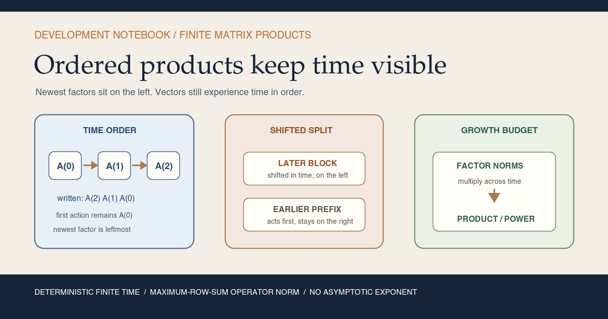
This is the proof-to-prose companion for
formalization/NonlinearDynamics/Random/MatrixProducts/FiniteProducts.lean.
It covers all thirteen public declarations in source order. There are no
private declarations in the module.
The preceding chapter, Finite Gaussian Unitary Ensemble Spectral Laws in Lean, completed the first finite random-matrix spectral-law interface. This chapter begins a different dependency branch: deterministic products first, then measurable random products and cocycles. The stable textbook treatments are Forward Matrix Product, Induced Infinity Operator Norm, and Ordered Finite Matrix Products and Operator-Norm Growth.
Choose a route up
| Route | Begin | Destination |
|---|---|---|
| First encounter | The recurrence behind the product | See why written order and action order point in opposite directions |
| Algebra route | The first four horizons | Read the recursion, split law, and constant-system power law |
| Dynamics route | Vectors experience chronological time | Connect matrix products to a nonautonomous orbit |
| Analysis route | Which norm is actually active? | Derive the maximum-row-sum induced norm and all four estimates |
| Lean route | The complete declaration map | Audit every public name and proof engine |
| Integrity route | Strict nonclaims | Separate finite deterministic control from random and asymptotic theory |
Learning objectives
By the summit, a reader should be able to:
- state the forward-product recurrence and its time-zero value;
- expand the horizons zero through three without reversing a factor;
- explain why the newest factor is written on the left;
- connect the written product to chronological matrix-vector action;
- state the shifted add-split theorem with the later block on the left;
- test that split at both boundary cases;
- recover ordinary matrix powers from a constant sequence;
- explain why the identity sequence stays the identity;
- distinguish the semiring assumptions from the analytic assumptions;
- identify the matrix norm selected by
Matrix.Norms.Operator; - distinguish that norm from Frobenius, spectral, and entrywise norms;
- explain exactly where positive dimension enters the current interface;
- prove a product-of-factor-norms upper bound by induction;
- pass from pointwise factor control to a power bound;
- explain why the power theorem needs no separate hypothesis \(0\le C\);
- transfer both matrix estimates to vector orbits;
- identify which real Jacobian and complex transfer-matrix applications share this interface;
- inspect all thirteen Lean declarations at the command line; and
- state what additional structure random or asymptotic theorems still need.
Lineage, contribution, and boundary
Ordered products of linear maps are standard in nonautonomous dynamics, derivative chains, transfer matrices, and random matrix theory. The classical random-product literature asks what happens after randomness, integrability, and long-time limits are added; Furstenberg and Kesten’s original product paper is one landmark (Furstenberg and Kesten, 1960). This chapter does not claim to invent finite product estimates or to formalize that asymptotic theory.
The local contribution is a small, declaration-complete Lean interface with one frozen time-order convention. It deliberately generalizes the algebraic core to arbitrary semiring scalars, so later real Jacobian chains and complex transfer matrices can share it. It then chooses one precise analytic norm and proves four finite-time upper bounds. The result is infrastructure, not a random-product theorem.
The recurrence behind the product
Let \(\iota\) be a finite coordinate type and let \(A_k\) be a square matrix whose rows and columns are indexed by \(\iota\). The source defines
\[ P_A(0)=I, \qquad P_A(k+1)=A_kP_A(k). \]The identity at zero is essential. It makes an empty product total, gives induction a clean base case, and says that advancing through no time steps changes no state. The successor rule prepends the newest factor. It does not append that factor on the right.
In Lean, the entire definition is a recursion on the horizon:
def forwardProduct (A : ℕ → Matrix ι ι 𝕜) : ℕ → Matrix ι ι 𝕜
  | 0 => 1
  | k + 1 => A k * forwardProduct A k
This definition uses no topology, norm, probability, or field division. A
Semiring 𝕜 supplies zero, one, addition, multiplication, and the
laws needed for finite matrix multiplication. Matrix multiplication can still
be noncommutative even when the scalar semiring is commutative.
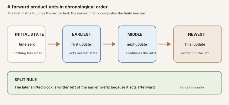
Figure: action proceeds from the initial vector through the earliest factor to the newest one. Written matrix composition therefore places the shifted later block on the left. The plate communicates order only; it does not assert randomness, invertibility, or long-time behavior.
The first four horizons
Unfolding the recursion once at a time gives the safest order audit:
\[ \begin{aligned} P_A(0) &{}= I,\\ P_A(1) &{}= A_0,\\ P_A(2) &{}= A_1A_0,\\ P_A(3) &{}= A_2A_1A_0. \end{aligned} \]Read the last line from right to left when it acts on a vector. The vector meets \(A_0\) first, then \(A_1\), then \(A_2\). The leftmost matrix is newest in time but last in action.
The first three public facts are almost definitionally exact:
forwardProduct_zeroexposes \(P_A(0)=I\);forwardProduct_succexposes \(P_A(k+1)=A_kP_A(k)\); andforwardProduct_onesimplifies the first nonempty horizon to \(A_0\).
The zero and successor theorems are marked @[simp]. They let
Lean’s simplifier reduce boundary values without reopening the definition in
every downstream proof.
Vectors experience chronological time
Suppose a state follows
\[ x_{k+1}=A_kx_k. \]Then the first steps are
\[ x_1=A_0x_0, \qquad x_2=A_1(A_0x_0), \qquad x_3=A_2(A_1(A_0x_0)). \]Associativity of matrix action turns the last expression into
\((A_2A_1A_0)x_0\). The theorem
forwardProduct_mulVec_succ records the one-step mechanism:
theorem forwardProduct_mulVec_succ
    (A : ℕ → Matrix ι ι 𝕜) (k : ℕ) (x : ι → 𝕜) :
    forwardProduct A (k + 1) *ᵥ x =
      A k *ᵥ (forwardProduct A k *ᵥ x)
The proof rewrites the successor product and then applies
Matrix.mulVec_mulVec, Mathlib’s matrix-action associativity law
(Mathlib matrix multiplication). Its companion
forwardProduct_mulVec_zero says that the zero-horizon identity
matrix leaves every vector fixed.
The source does not define a separate orbit object here. It gives later orbit modules the exact algebraic facts needed to build one without committing this foundational file to a particular state-space abstraction.
Splitting time without reversing it
A useful product must be splittable. Fix an earlier horizon \(m\), then take another \(k\) steps. Define the shifted sequence
\[ A^{(m)}_j=A_{m+j}. \]The exact concatenation law is
\[ P_A(m+k)=P_{A^{(m)}}(k)P_A(m). \]The earlier prefix \(P_A(m)\) sits on the right because it acts first. The later shifted block sits on the left because it acts afterward. For \(m=2\) and \(k=3\), the theorem reads
\[ A_4A_3A_2A_1A_0 = (A_4A_3A_2)(A_1A_0). \]This concrete expansion is the quickest test of any proposed split formula. A formula placing \(P_A(m)\) on the left is wrong for the chosen convention unless all factors happen to commute.
The public theorem is forwardProduct_add:
theorem forwardProduct_add (A : ℕ → Matrix ι ι 𝕜) (m k : ℕ) :
    forwardProduct A (m + k) =
      forwardProduct (fun j => A (m + j)) k * forwardProduct A m
The name follows the natural-number argument being split. Its documentation states the semantic content: split after \(m\) steps, shift the later block, and keep that block on the left.
Both boundary tests matter
If \(k=0\), the later block is the identity:
\[ P_A(m+0)=IP_A(m)=P_A(m). \]If \(m=0\), the shifted sequence is the original sequence:
\[ P_A(0+k)=P_A(k)I=P_A(k). \]The Lean proof inducts on \(k\). The base case is simplification. The successor
case uses Nat.add_succ, unfolds both successor products, substitutes
the induction hypothesis, and closes with associativity. It never commutes
matrix factors.
The split theorem and Matrix.mulVec_mulVec immediately derive the
useful vector identity
That identity is intentionally not another public theorem in this minimal slice. It is an exercise in composing the two exported interfaces.
Constant systems recover powers
If every time step uses one fixed matrix \(B\), the nonautonomous notation
should collapse to the familiar autonomous one. The theorem
forwardProduct_const proves
The proof is another induction. Its successor step has the left-recursive
shape \(BB^k\), so it uses Mathlib’s pow_succ’ orientation. No
commutativity of arbitrary matrices is assumed; every factor is the same
matrix.
Setting \(B=I\) gives
\[ P_{j\mapsto I}(k)=I. \]The source keeps that corollary as the named theorem
forwardProduct_const_one. Although simplification can already
derive it from forwardProduct_const, the explicit name is a useful
consistency check and a discoverable interface for identity dynamics.
An assumption ledger with two floors
The file is organized so algebra does not inherit analysis accidentally.
| Layer | Lean assumptions | What they buy | What they do not buy |
|---|---|---|---|
| Shared matrix shape | [Fintype ι] [DecidableEq ι] | Finite index enumeration and decidable diagonal equality used by multiplication and identity | A chosen numerical dimension or an ordering of coordinates |
| Algebra | [Semiring 𝕜] | Products, powers, identities, and matrix-vector action | Subtraction, division, topology, norms, probability |
| Analysis | [RCLike 𝕜] [Nonempty ι] | Real-or-complex normed-field structure and normalized identity norm in positive finite dimension | Randomness, measurability, invertibility, limits |
The generic scalar parameter matters. Real Jacobian chains naturally use
\(\mathbb R\), while quantum or wave transfer matrices often use
\(\mathbb C\). Both share the same algebraic recursion. The
RCLike typeclass covers precisely those two analytic scalar
settings for this module’s norm proofs.
The source also does not force \(\iota=\operatorname{Fin}(n)\). Any finite coordinate type works. That flexibility lets later modules use structured finite indices without reindexing every matrix before taking a product.
Which norm is actually active?
Matrix notation such as \(\lVert A\rVert\) is ambiguous until a norm scope is fixed. This file opens
open scoped BigOperators Matrix Matrix.Norms.Operator
The final scope selects Mathlib’s induced infinity operator norm. For a vector \(x:\iota\to\mathbb K\), the function-space norm is the supremum norm
\[ \lVert x\rVert_\infty=\max_{i\in\iota}|x_i|. \]For a matrix \(A\), the induced norm is the maximum absolute row sum
\[ \lVert A\rVert_{\infty\to\infty} = \max_{i\in\iota}\sum_{j\in\iota}|A_{ij}|. \]Mathlib implements the same quantity as an outer finite supremum of inner row
sums and proves that it agrees with the operator norm of the corresponding
continuous linear map. The exact pinned API lives in
Mathlib.Analysis.Matrix.Normed
(official documentation).
Four nearby norms that are not interchangeable
| Name | Typical expression | Is it active here? |
|---|---|---|
| Maximum-row-sum induced norm | (\max_i\sum_j | A_{ij} |
| Euclidean spectral operator norm | largest singular value | No |
| Frobenius norm | ((\sum_{i,j} | A_{ij} |
| Entrywise maximum | (\max_{i,j} | A_{ij} |
The words “operator norm” alone are not enough. An operator norm depends on the vector norms in its domain and codomain. Here both are supremum norms, so the resulting matrix formula is a maximum row sum. A future theorem under a Euclidean operator-norm scope would be a distinct result and should have a distinct name.
Why positive dimension is visible
The analytic section assumes [Nonempty ι]. In a nonempty finite
coordinate space, the identity operator has norm one:
That normalization closes the time-zero base case of the product bound. In
Mathlib, the relevant NormOneClass instance for this matrix norm
also carries the Nonempty assumption, so the Lean interface makes
it visible rather than relying on a hidden dimension convention.
An empty index type behaves differently. There is only one empty square
matrix; its identity and zero matrices coincide, and the finite row supremum
is zero. The upper inequalities are not thereby mathematically false. Rather,
the current analytic API chooses the familiar normalized identity statement
\(\lVert I\rVert=1\), so it works in positive finite dimension. This chapter
does not claim Nonempty is the weakest conceivable assumption for
every inequality.
Bound one: multiply the factor norms
Submultiplicativity says
\[ \lVert AB\rVert_{\infty\to\infty} \le \lVert A\rVert_{\infty\to\infty} \lVert B\rVert_{\infty\to\infty}. \]Induction on the recurrence then yields
\[ \lVert P_A(k)\rVert_{\infty\to\infty} \le \prod_{j\lt k}\lVert A_j\rVert_{\infty\to\infty}. \]This is linfty_opNorm_forwardProduct_le_prod. Its proof has four
moves:
- at zero, simplify the identity norm and the empty scalar product to one;
- at a successor, rewrite \(P_A(k+1)=A_kP_A(k)\);
- apply matrix-norm submultiplicativity and the induction hypothesis; and
- commute only the two nonnegative real norm factors so the expression
matches
Finset.prod_range_succ.
The fourth move is easy to misread. The proof never claims \(A_kP_A(k)=P_A(k)A_k\). Matrices remain ordered. Their norms are real numbers, and multiplication of those scalar bounds is commutative.
Bound two: a uniform prefix budget becomes a power
Assume every factor used before horizon \(k\) obeys
\[ \forall j\lt k,\qquad \lVert A_j\rVert_{\infty\to\infty}\le C. \]Termwise comparison of the finite scalar products gives
\[ \prod_{j\lt k}\lVert A_j\rVert_{\infty\to\infty} \le \prod_{j\lt k} C = C^k. \]Composing this with the first bound produces
\[ \lVert P_A(k)\rVert_{\infty\to\infty}\le C^k. \]The theorem is linfty_opNorm_forwardProduct_le_pow. Notice that
its hypothesis controls only the prefix actually used. It does not require a
global assertion about \(A_j\) for all future times.
Why there is no separate nonnegativity hypothesis on \(C\)
The theorem does not assume \(0\le C\). That omission is mathematically sound.
- If \(k=0\), the factor hypothesis is vacuous and \(C^0=1\) for every real \(C\). The claim is \(\lVert I\rVert\le1\).
- If \(k\gt0\), then \(j=0\) lies in the controlled prefix. Since norms are nonnegative and \(\lVert A_0\rVert\le C\), the hypothesis itself forces \(C\ge0\).
Lean’s proof can pass directly through Finset.prod_le_prod using
factor nonnegativity and the supplied pointwise inequalities. Adding a
separate 0 ≤ C argument would be redundant for positive horizons
and unnecessarily restrictive at the empty horizon.
Bounds three and four: control every vector orbit
The induced norm is designed to control action:
\[ \lVert Ax\rVert_\infty \le \lVert A\rVert_{\infty\to\infty}\lVert x\rVert_\infty. \]Apply that inequality with \(A=P_A(k)\), then substitute either matrix bound. The result is
\[ \lVert P_A(k)x\rVert_\infty \le \left(\prod_{j\lt k}\lVert A_j\rVert_{\infty\to\infty}\right) \lVert x\rVert_\infty, \]exported as
linfty_opNorm_forwardProduct_mulVec_le_prod, and
exported as
linfty_opNorm_forwardProduct_mulVec_le_pow under the same prefix
hypothesis.
Both proofs begin with Matrix.linfty_opNorm_mulVec. They multiply
the previously established matrix inequality by the nonnegative number
\(\lVert x\rVert\). Nothing in either theorem supplies a matching lower bound
or says that the estimate is sharp.
What the bounds mean for dynamics
For a differentiable discrete system, a derivative along an orbit often forms a chain
\[ Df(x_{k-1})\cdots Df(x_1)Df(x_0). \]The order is exactly the forward convention. The finite product estimates can therefore become one ingredient in later stability or sensitivity theorems. But this module does not define derivatives, choose an orbit, or infer stability from an upper bound. In particular, \(C\gt1\) permits growth, and an upper estimate with \(C\lt1\) becomes a contraction statement only after the later theorem supplies the relevant hypotheses and interpretation.
For a constant matrix \(B\), the power theorem reduces to the familiar estimate \(\lVert B^k\rVert\le\lVert B\rVert^k\). For a genuinely time-dependent system, the product-of-norms theorem retains the individual finite-time budget and can be much more informative than replacing every factor by one worst-case constant.
The complete declaration map
The module exports exactly thirteen public declarations and no private helper. The table follows source order.
| Declaration | Assumption floor | Exact role | Proof engine |
|---|---|---|---|
forwardProduct | Semiring 𝕜 | Defines the identity-at-zero, newest-factor-left product | Recursion on the natural horizon |
forwardProduct_zero | Semiring 𝕜 | Exposes the empty product as the identity | Definitional equality |
forwardProduct_succ | Semiring 𝕜 | Exposes the successor recurrence | Definitional equality |
forwardProduct_add | Semiring 𝕜 | Splits after \(m\) steps with the shifted later block on the left | Induction on the later length and associativity |
forwardProduct_one | Semiring 𝕜 | Computes the one-step product as \(A_0\) | Simplification of the recurrence |
forwardProduct_const | Semiring 𝕜 | Identifies a constant matrix sequence with ordinary powers | Induction and pow_succ’ |
forwardProduct_const_one | Semiring 𝕜 | Shows the identity sequence stays identity | Constant theorem and simplification |
forwardProduct_mulVec_zero | Semiring 𝕜 | Shows the zero-horizon product fixes every vector | Identity matrix action |
forwardProduct_mulVec_succ | Semiring 𝕜 | Reassociates successor product action into chronological action | Matrix.mulVec_mulVec |
linfty_opNorm_forwardProduct_le_prod | RCLike 𝕜, Nonempty ι | Bounds product norm by the finite product of factor norms | Induction, submultiplicativity, and scalar monotonicity |
linfty_opNorm_forwardProduct_le_pow | RCLike 𝕜, Nonempty ι | Converts a uniform prefix bound into \(C^k\) | Finite-product comparison |
linfty_opNorm_forwardProduct_mulVec_le_prod | RCLike 𝕜, Nonempty ι | Transfers the factor-product estimate to every vector | Induced operator-norm action bound |
linfty_opNorm_forwardProduct_mulVec_le_pow | RCLike 𝕜, Nonempty ι | Transfers the uniform power estimate to every vector | Induced action bound and the preceding power theorem |
The namespace is
NonlinearDynamics.Random.MatrixProducts. The presence of
Random in the namespace locates the future application branch; it
does not make any declaration in this file probabilistic.
Lean proof engineering
Why recurse on the horizon rather than a finite list?
The intended downstream object is a time-indexed family \(A:\mathbb N\to \operatorname{Matrix}\). Recursion on \(k\) makes the factor at the newest time available exactly where the successor equation needs it. A list product could encode the same finite sequence, but it would require repeated conversion between natural-time indexing, prefixes, and list reversal.
Why is the split theorem proved by induction on the later block?
Holding \(m\) fixed makes the shift \(j\mapsto m+j\) stable. Each successor adds exactly the next matrix \(A_{m+k}\) to the left. Inducting on the earlier block would obscure that chronological step and complicate the shifted index.
Why are the norm theorem names long?
The prefix linfty_opNorm is claim discipline. Matrix norms are not
unique, and later work may need Frobenius or Euclidean spectral estimates. The
name prevents a downstream reader from silently importing a stronger norm
interpretation than Lean proved.
Why use RCLike rather than hard-code complex matrices?
The algebraic recursion is shared by real and complex dynamics. The analytic
proofs need standard absolute values, normed-field structure, and the Mathlib
matrix norm instances. RCLike supplies that common real-or-complex
surface without duplicating four theorems.
Why does the product proof commute something at the end?
Finset.prod_range_succ presents the new scalar factor at one end,
while submultiplicativity naturally produces it at the other. The proof uses
mul_comm only after matrices have become real norms. Matrix order
never changes.
Why not export every easy corollary?
Two-step expansion, vector splitting, the zero-horizon norm, and constant vector bounds are all short consequences. Keeping them out of this first API reduces maintenance while the foundational convention settles. A later module should add a named corollary when a real downstream proof repeatedly needs it, not merely because it is provable.
How to run the checked source
Compile the module directly with every warning promoted to an error:
source "$HOME/.elan/env"
cd formalization
lake env lean -DwarningAsError=true \
  NonlinearDynamics/Random/MatrixProducts/FiniteProducts.lean
Build the complete Lean library:
source "$HOME/.elan/env"
cd formalization
lake build
From the repository root, check the public teaching content:
make content-hygiene
make site-check
This import-level snippet checks all thirteen public declarations:
import NonlinearDynamics.Random.MatrixProducts.FiniteProducts

open scoped BigOperators Matrix Matrix.Norms.Operator
open NonlinearDynamics.Random.MatrixProducts

#check forwardProduct
#check forwardProduct_zero
#check forwardProduct_succ
#check forwardProduct_add
#check forwardProduct_one
#check forwardProduct_const
#check forwardProduct_const_one
#check forwardProduct_mulVec_zero
#check forwardProduct_mulVec_succ
#check linfty_opNorm_forwardProduct_le_prod
#check linfty_opNorm_forwardProduct_le_pow
#check linfty_opNorm_forwardProduct_mulVec_le_prod
#check linfty_opNorm_forwardProduct_mulVec_le_pow
Save the snippet inside formalization and run
lake env lean path/to/Scratch.lean.
Useful local Mathlib reconnaissance:
rg -n "linfty_opNorm_def|linfty_opNorm_mul|linfty_opNorm_mulVec" \
  formalization/.lake/packages/mathlib/Mathlib/Analysis/Matrix/Normed.lean

rg -n "mulVec_mulVec" \
  formalization/.lake/packages/mathlib/Mathlib/Data/Matrix/Mul.lean
The pinned local Mathlib 4.32.0 release checkout is the exact API authority. Online documentation is a navigation aid, not a replacement for compiling against the selected source.
Common failure modes
Appending the newest factor on the right
Defining \(P_A(k+1)=P_A(k)A_k\) is internally consistent but does not match the chronological column-vector action used here. It makes \(A_k\) act first on a vector. Audit \(P_A(3)\) before proving anything downstream.
Putting the earlier prefix on the left in the split
The wrong formula often looks plausible because scalar multiplication is commutative. Matrix multiplication is not. Expand the \(m=2,k=3\) example: the later block must be \(A_4A_3A_2\) on the left.
Commuting matrices because their norms commute
The norm proof ends with a scalar mul_comm. That licenses only a
reordering of real upper-bound factors. It says nothing about the underlying
matrices.
Calling the active norm spectral or Frobenius
The selected norm is maximum row sum, induced by vector supremum norms. Singular-value and Frobenius arguments live under different definitions and scopes.
Hiding the empty-index boundary
The analytic theorems assume Nonempty ι so the identity norm is
one. Deleting that hypothesis without redesigning the base case confuses the
empty matrix space with ordinary positive dimension.
Adding a redundant hypothesis \(0\le C\)
The existing theorem is stronger at horizon zero and already forces
nonnegativity at every positive horizon. A downstream corollary may carry
0 ≤ C because it is convenient, but it should not be reported as
an assumption of this declaration.
Reading the prefix hypothesis globally
∀ j < k, ‖A j‖ ≤ C controls exactly the factors appearing in
\(P_A(k)\). It makes no statement about \(A_k,A_{k+1},\ldots\).
Turning an upper bound into an exponent
A finite inequality is not a limit. Taking logarithms may fail when a product norm is zero, and dividing by time does not prove convergence. Random and ergodic hypotheses are entirely absent.
Treating the namespace as a theorem assumption
The file lives under Random.MatrixProducts because that is one
planned consumer. Its inputs are ordinary deterministic matrix sequences.
No sample space appears in any declaration.
Strict nonclaims
This module proves a deterministic finite-time interface. It does not prove or define:
- a random matrix sequence, probability law, measurable matrix process, independence, stationarity, or expectation;
- a base dynamical system, shift map, or measurable cocycle equation;
- invertibility, negative time, or a two-sided product;
- logarithms of norms, including any convention for a zero product;
- a subadditive limit, limsup formula, or almost-sure growth rate;
- a Lyapunov exponent, Lyapunov splitting, Furstenberg-Kesten theorem, or multiplicative ergodic theorem;
- a lower growth bound, equality case, sharpness result, contraction theorem, or stability conclusion;
- spectral-radius, eigenvalue, singular-value, determinant, or trace control;
- a Frobenius-norm or Euclidean spectral-norm estimate;
- an equivalence between different finite-dimensional norms;
- convergence of an infinite product;
- rectangular matrix products with changing intermediate index types;
- commutativity, Hermiticity, normality, unitarity, positivity, or symplectic structure of the factors; or
- a numerical multiplication algorithm, conditioning estimate, or rounding error analysis.
The four exported inequalities are upper bounds in one named norm. They are building blocks for later theorems, not substitutes for those theorems.
Exercises with solutions
Exercise 1: expand the recurrence
Write \(P_A(4)\) without product notation.
Solution.
\[ P_A(4)=A_3A_2A_1A_0. \]Each successor adds the newest factor on the left.
Exercise 2: follow a vector
In what order do the factors of \(P_A(4)\) act on \(x\)?
Solution. \(A_0\) acts first, then \(A_1\), then \(A_2\), then \(A_3\). Written order is the reverse of action order.
Exercise 3: audit a shifted split
Expand the split theorem at \(m=1\) and \(k=3\).
Solution.
\[ P_A(4)=(A_3A_2A_1)A_0. \]The shifted sequence begins at time one, and its three-step product is the left block.
Exercise 4: derive vector splitting
Combine forwardProduct_add with
Matrix.mulVec_mulVec.
Solution. If \(A^{(m)}_j=A_{m+j}\), then
\[ P_A(m+k)x=P_{A^{(m)}}(k)(P_A(m)x). \]The earlier prefix acts first.
Exercise 5: specialize to a constant matrix
What does the split theorem become when \(A_j=B\) for every \(j\)?
Solution. It becomes
\[ B^{m+k}=B^kB^m. \]Because both factors are powers of the same matrix, this agrees with the usual power law.
Exercise 6: compute the active norm
For the real matrix
\[ A=\begin{pmatrix}1&-2\\3&4\end{pmatrix}, \]what is the maximum-row-sum operator norm?
Solution. The absolute row sums are \(1+2=3\) and \(3+4=7\), so \(\lVert A\rVert_{\infty\to\infty}=7\). This calculation does not compute the Euclidean spectral norm.
Exercise 7: apply the product bound
Suppose the first three factor norms are at most \(2\), \(1/2\), and \(3\). What finite-time upper bound follows for \(\lVert P_A(3)\rVert\)?
Solution. The product theorem gives at most \(2\cdot(1/2)\cdot3=3\). Replacing every factor by the worst bound \(3\) would give \(27\), which is valid but less informative.
Exercise 8: explain the sign of \(C\)
Could the hypotheses of the power theorem hold with \(k=2\) and \(C=-1\)?
Solution. No. They would include \(\lVert A_0\rVert\le-1\), contradicting nonnegativity of norms. At \(k=0\), however, the factor hypothesis is empty and the theorem correctly allows any \(C\).
Exercise 9: transfer to a state
If \(\lVert A_j\rVert\le0.9\) for every \(j\lt k\), what does the final theorem say about a vector \(x\)?
Solution. It says
\[ \lVert P_A(k)x\rVert_\infty\le0.9^k\lVert x\rVert_\infty. \]The module itself does not package this as a nonlinear stability theorem.
Exercise 10: identify the assumption floor
Which declarations remain available for matrices over the natural numbers?
Solution. All nine algebraic declarations, from
forwardProduct through forwardProduct_mulVec_succ, use
only a semiring. The four analytic norm declarations require
RCLike, so they do not apply to natural-number scalars as stated.
Exercise 11: inspect dimension zero
Why is Nonempty ι not present on forwardProduct_zero?
Solution. The algebraic identity exists even for the empty matrix type. Positive dimension is introduced only when the analytic layer wants the standard normalized identity norm at its induction base.
Exercise 12: test an overclaim
Does \(\lVert P_A(k)\rVert\le C^k\) prove that \(k^{-1}\log\lVert P_A(k)\rVert\) converges?
Solution. No. The norm may vanish, the logarithm then needs a convention, and one upper estimate gives neither existence nor identification of a limit. Random-product and ergodic theorems require substantial additional structure.
The next ridge
The ordered finite product is now stable enough to serve several branches.
One branch can define matrix cocycles over a base transformation and prove the
finite cocycle equation from forwardProduct_add. Another can make
the matrix sequence random, prove measurability of every finite product, and
state integrability hypotheses for logarithmic norms. The deterministic branch
can reuse the same order for Jacobian chains in finite-time stability and
sensitivity estimates.
The dependency order matters. A measurable random product needs this product map first. A Lyapunov-growth theorem additionally needs a logarithmic observable, zero handling, integrability, and a limit theorem. A multiplicative ergodic theorem needs still more, including a base dynamical system and the hypotheses that support invariant asymptotic subspaces. None of those layers should be inferred from the four bounds proved here.
The immediate successor, Measurable Finite Matrix Products in Lean, lifts this convention outcome by outcome, proves measurability from exactly the used factor prefix, and defines proof-carrying pushforward laws with a mass-one probability wrapper. It remains finite-time and introduces no independence, factorization, cocycle, or asymptotic claim.
References
The links below were checked on 2026-07-21. The pinned local Mathlib 4.32.0 checkout remains the exact API authority for the Lean proof.
Mathlib contributors.
Mathlib 4.32.0 release,
2026. This is the dependency release selected by
formalization/lakefile.toml.
Mathlib contributors.
Matrix multiplication,
Mathlib 4 documentation. This official page defines matrix multiplication,
Matrix.mulVec, and Matrix.mulVec_mulVec, the action
associativity theorem used by the vector recursion.
Mathlib contributors.
Matrices as normed spaces,
Mathlib 4 documentation. This official page defines the maximum-row-sum matrix
norm under Matrix.Norms.Operator, proves matrix
submultiplicativity and the matrix-vector estimate, supplies the positive-
dimension identity normalization, and identifies the matrix norm with the
corresponding continuous-linear-map operator norm.
Harry Furstenberg and Harry Kesten. “Products of Random Matrices”, The Annals of Mathematical Statistics 31(2), 457-469, 1960. This original paper is cited only as historical context for the later random and asymptotic program. The present Lean module proves no theorem from that paper.