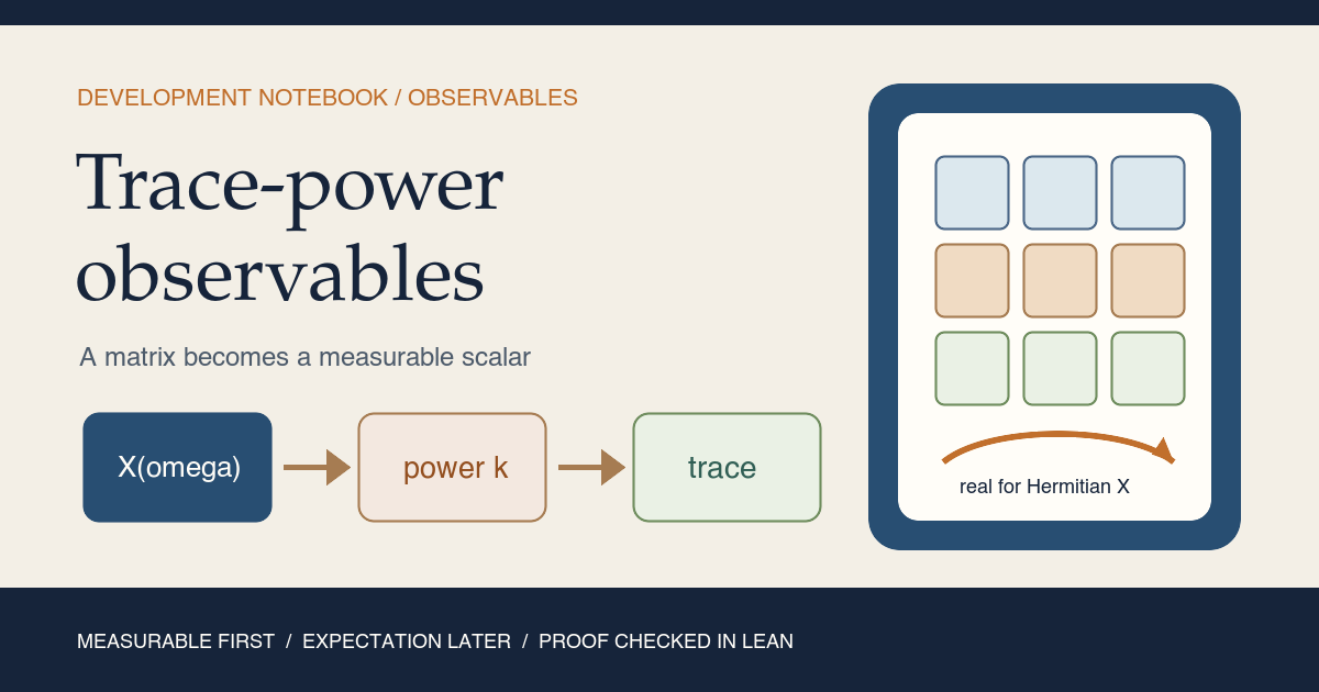
Suppose a random experiment produces a square matrix \(X(\omega)\). One outcome might produce one matrix, another outcome a different matrix. Even in finite dimensions, the whole matrix is often the wrong scale at which to ask a probabilistic question. We want a scalar summary that is sensitive to the collective action of the entries.
The trace of a matrix power is one of the first such summaries:
\[ S_k(\omega)=\operatorname{tr}\!\left(X(\omega)^k\right). \]The matrix \(X(\omega)\) is a realization. The natural number \(k\) chooses a
power. The output \(S_k(\omega)\) is one complex number. As \(\omega\) varies,
\(S_k\) is initially only a scalar-valued map. Once \(X\) is assumed
measurable and measurable_tracePower is applied, it becomes a scalar random
observable in the standard measure-theoretic sense.
This module establishes two facts before doing any averaging:
- if \(X\) is measurable, then \(S_k\) is measurable;
- if every realization of \(X\) is Hermitian, then \(S_k(\omega)\) is real for every outcome, with an almost-sure version for almost-sure Hermiticity.
That order matters. A formula can look like a moment without yet being one. Expectation needs a measure, and a mathematically meaningful finite moment needs an integrability argument. This file assumes neither.
Choose a route up
| Route | Start at | You will leave with |
|---|---|---|
| First encounter | Why trace? | A concrete picture of what \(\operatorname{tr}(X^k)\) records |
| Probability route | Measurability | The exact closure argument from matrix entries to a scalar random variable |
| Linear algebra route | Hermitian reality | A proof that every trace power lies on the real axis |
| Lean route | Declaration map | Every definition and theorem in Observables.lean, with its proof design |
| Research route | Moment method | The precise bridge from trace powers to expected spectral moments, plus the missing hypotheses |
Learning objectives
By the summit, you should be able to:
- distinguish a realized matrix, a trace-power observable, and its expected trace moment;
- derive the trace powers of diagonal and two-by-two Hermitian matrices;
- explain why finite matrix multiplication and trace preserve measurability;
- read a natural-number induction proof in Lean;
- explain why Hermitian matrix powers remain Hermitian;
- move cleanly between pointwise and almost-everywhere statements; and
- identify every ingredient still missing from a formal moment-method proof.
The ascent in one picture
flowchart LR
  A[Outcome omega] --> B[Matrix X of omega]
  B --> C[Power X of omega to k]
  C --> D[Trace-power scalar S k of omega]
  M[Measurable X] --> P[Measurable matrix power]
  P --> Q[Measurable trace power]
  H[Hermitian X] --> R[Hermitian matrix power]
  R --> T[Trace power has zero imaginary part]
  U[Probability measure and integrability] -. future work .-> V[Expected trace moment]
  D --> V
Reading the route. The solid paths are formalized in Observables.lean. The dotted path is deliberately absent: the current file defines the pointwise observable but does not choose a probability measure, prove integrability, or take an expectation.
Where this entry begins
The preceding Knowledge Base chapter, Random Matrices: From Outcomes to Spectra, builds the lower mountain: sample spaces, entrywise measurability, matrix operations, conjugate transpose , and Hermitian symmetry . This notebook entry starts from that established interface and follows the next Lean file closely.
The recurring vocabulary is already indexed in the Knowledge Base:
| Term | Working meaning here |
|---|---|
| Random matrix | A measurable map from outcomes to matrices, once measurability has been supplied |
| Measurable space | The event structure needed to state that a map is measurable |
| Hermitian matrix | A square complex matrix satisfying \(H^*=H\) |
| Almost everywhere | A property allowed to fail only on a set of measure zero |
What this entry contributes
This is a teaching account of an implementation, not a novelty claim. The mathematics of traces, Hermitian powers, and spectral moments is classical. The local contribution is narrower:
- one reusable definition of a trace-power observable;
- a measurable-power induction built on the project’s matrix multiplication lemma;
- measurable trace powers for arbitrary finite index types;
- pointwise and almost-sure reality statements for Hermitian inputs; and
- a bundled API that lets later ensemble files reuse those facts without unpacking record fields by hand.
Not claimed
- No Gaussian ensemble, entry distribution, independence hypothesis, or normalization convention is defined here.
- No expectation or integral is taken.
- No integrability or finite-moment hypothesis is proved.
- No spectral theorem, eigenvalue identity, unitary invariance, semicircle law, or asymptotic limit is formalized in this module.
Base camp: why compress a matrix?
For a finite square matrix \(A=(A_{ij})\), the trace is the sum of the diagonal entries:
\[ \operatorname{tr}(A)=\sum_i A_{ii}. \]That definition looks coordinate-dependent, but trace has a deeper role. It is unchanged by a change of basis of the form \(A\mapsto UAU^{-1}\). For a Hermitian matrix, the spectral theorem diagonalizes \(A\), and trace becomes the sum of its real eigenvalues. The current Lean file does not prove those spectral facts, but they explain why trace is the right scalar to preserve (Mathlib trace API; Mathlib Hermitian spectrum API).
Now apply trace after a matrix power:
\[ \operatorname{tr}(A^k). \]If \(A\) has eigenvalues \(\lambda_i\), then the spectral picture predicts
\[ \operatorname{tr}(A^k)=\sum_i \lambda_i^k. \]Each power asks a different question of the spectrum. Low powers capture broad features such as total location and quadratic scale. Higher powers become more sensitive to eigenvalues far from the origin. This is the runway to the moment method, but it is not yet the moment method itself.
A diagonal worked example
Let
\[ D=\operatorname{diag}(\lambda_1,\ldots,\lambda_n). \]Powers of a diagonal matrix are computed entrywise:
\[ D^k=\operatorname{diag}(\lambda_1^k,\ldots,\lambda_n^k). \]Therefore
\[ \operatorname{tr}(D^k)=\lambda_1^k+\cdots+\lambda_n^k. \]This is the cleanest mental model for a trace-power observable. A general Hermitian matrix is not already diagonal, but unitary diagonalization gives the same spectral interpretation.
A two-by-two Hermitian worked example
Write the general two-by-two Hermitian matrix as
\[ H= \begin{bmatrix} a & z \\ \overline z & b \end{bmatrix}, \qquad a,b\in\mathbb R,\quad z\in\mathbb C. \]The first trace power is immediate:
\[ \operatorname{tr}(H)=a+b. \]For the second power,
\[ H^2= \begin{bmatrix} a^2+z\overline z & az+zb \\ \overline z a+b\overline z & \overline z z+b^2 \end{bmatrix}. \]Taking the trace gives
\[ \operatorname{tr}(H^2)=a^2+b^2+2|z|^2. \]The expression is visibly real. The Lean proof will not expand entries like this. It proves a structural theorem once: powers preserve Hermiticity, and the trace of a Hermitian matrix is fixed by conjugation.
Camp one: the pointwise observable is not an expectation
The core definition is short:
/-- The `k`th trace-power observable of a square complex random matrix. -/
def tracePower [Fintype ι] [DecidableEq ι]
    (X : RandomMatrix Ω ι ι ℂ) (k : ℕ) : Ω → ℂ :=
  fun ω ↦ Matrix.trace ((X ω) ^ k)
Read the type from right to left:
Ω → ℂsays the output is a complex-valued function of the sample;k : ℕselects the matrix power;X : RandomMatrix Ω ι ι ℂis a square complex matrix-valued map;[Fintype ι]says the row and column index set is finite; and[DecidableEq ι]lets Lean construct the identity matrix used by natural powers.
The definition makes no measurability claim by itself. In this project,
RandomMatrix is the underlying map type. A separate theorem carries the
proof that the map is measurable.
Most importantly, the definition contains no measure:
\[ \texttt{tracePower X k}:\Omega\to\mathbb C. \]An expectation would additionally require a measure \(\mu\) on \(\Omega\):
\[ \mathbb E_\mu[S_k] =\int_\Omega \operatorname{tr}(X(\omega)^k)\,d\mu(\omega). \]That integral is not tracePower. It consumes tracePower later. Mathlib’s
average API likewise keeps the measure-theoretic average distinct from the
integrability lemmas needed to reason about it
(Mathlib average API).
Pointwise, random, and averaged: keep the levels separate
| Object | Formula | What has been formalized here? |
|---|---|---|
| Realized matrix | \(X(\omega)\) | The input at one outcome |
| Realized scalar | \(\operatorname{tr}(X(\omega)^k)\) | Yes, by tracePower |
| Scalar random observable | \(\omega\mapsto\operatorname{tr}(X(\omega)^k)\) | Yes, with measurability proved |
| Expected trace moment | \(\mathbb E_\mu[\operatorname{tr}(X^k)]\) | No |
| Normalized expected trace moment | \(n^{-1}\mathbb E_\mu[\operatorname{tr}(X^k)]\) | No |
| Limiting spectral moment | A limit as matrix dimension grows | No |
Camp two: proving the observable is measurable
Trace power is a composition of two operations:
- raise a random matrix to the \(k\)th power;
- take the trace.
The proof mirrors that decomposition. First prove matrix powers are measurable. Then reuse the earlier theorem that trace is measurable.
The measurable-power theorem
/-- Pointwise matrix powers preserve measurability in finite dimensions. -/
theorem measurable_matrixPow [Fintype ι] [DecidableEq ι]
    {X : RandomMatrix Ω ι ι ℂ} (hX : Measurable X) (k : ℕ) :
    Measurable fun ω ↦ (X ω) ^ k := by
  induction k with
  | zero =>
      simpa only [pow_zero] using
        (measurable_const (Ω := Ω) (1 : Matrix ι ι ℂ))
  | succ k ih =>
      simpa only [pow_succ] using measurable_mul ih hX
The proof is induction on the natural number \(k\). This is exactly the right
proof shape because powers are recursively generated by a base case and a
successor case. Lean’s official theorem-proving text presents the same zero
and succ architecture for natural-number induction
(Lean induction and recursion):
Lean exposes the same two branches.
Zero branch
At power zero, the random matrix disappears from the value:
\[ \omega\longmapsto X(\omega)^0=I. \]This is a constant matrix-valued function. The earlier Basic module already
proved that constant matrices are measurable. The expression
The type annotation in (1 : Matrix ι ι ℂ) disambiguates the multiplicative identity.
simpa only [pow_zero] performs one controlled simplification. It rewrites the
goal using the rule \(X^0=1\) and checks that the previously proved constant
measurability theorem has the resulting type.
Successor branch
The induction hypothesis ih says
Measurable fun ω ↦ (X ω) ^ k
and hX says the original matrix map is measurable. The earlier theorem
measurable_mul ih hX combines them pointwise:
Finally, simpa only [pow_succ] identifies that product with
\(X(\omega)^{k+1}\).
The measurable trace-power theorem
/-- Every trace-power observable of a measurable finite random matrix is
measurable. -/
theorem measurable_tracePower [Fintype ι] [DecidableEq ι]
    {X : RandomMatrix Ω ι ι ℂ} (hX : Measurable X) (k : ℕ) :
    Measurable (tracePower X k) := by
  change Measurable fun ω ↦ Matrix.trace ((X ω) ^ k)
  exact measurable_trace (measurable_matrixPow hX k)
This proof has two moves.
First, change unfolds the public name just enough to show Lean the function
that must be measurable. It does not rewrite the entire goal indiscriminately.
Second, measurable_matrixPow hX k proves that the matrix-valued power is
measurable. The previously established measurable_trace theorem then turns a
measurable finite matrix into a measurable scalar trace.
Mathematically, trace is a finite sum of diagonal coordinates:
\[ \omega\longmapsto \sum_i \bigl(X(\omega)^k\bigr)_{ii}. \]Every diagonal coordinate is measurable, and a finite sum of measurable complex functions is measurable. The one-line Lean proof uses no probability assumption.
High camp: why Hermitian trace powers are real
A complex matrix can have a complex trace. The module keeps the codomain \(\mathbb C\), then proves the imaginary part vanishes under a Hermitian hypothesis.
This is a structural two-step argument:
- if \(H\) is Hermitian, then \(H^k\) is Hermitian;
- the trace of a Hermitian matrix is fixed by complex conjugation, so its imaginary part is zero.
Powers preserve pointwise Hermiticity
omit [MeasurableSpace Ω] in
/-- Every power of an everywhere-Hermitian finite random matrix remains
Hermitian everywhere. -/
theorem IsHermitianEverywhere.matrixPow [Fintype ι] [DecidableEq ι]
    {X : RandomMatrix Ω ι ι ℂ} (hX : IsHermitianEverywhere X) (k : ℕ) :
    IsHermitianEverywhere fun ω ↦ (X ω) ^ k :=
  fun ω ↦ (hX ω).pow k
IsHermitianEverywhere X means
Once an outcome \(\omega\) is fixed, hX ω is an ordinary Mathlib proof that
the matrix \(X(\omega)\) is Hermitian. Mathlib’s Matrix.IsHermitian.pow
theorem returns a proof that \(X(\omega)^k\) is Hermitian. The function
fun ω ↦ ... performs that same argument for every outcome
(Mathlib Hermitian API).
Notice the wrapper:
omit [MeasurableSpace Ω] in
It records an important dependency fact. This theorem is purely algebraic. It does not inspect events, measures, or measurable functions, so the measurable space on \(\Omega\) should not appear among its logical assumptions.
Why the trace lands on the real axis
For any finite matrix \(A\), conjugate transpose interacts with trace as
\[ \operatorname{tr}(A^*) =\overline{\operatorname{tr}(A)}. \]If \(A\) is Hermitian, then \(A^*=A\), hence
\[ \overline{\operatorname{tr}(A)} =\operatorname{tr}(A). \]A complex number equals its conjugate exactly when its imaginary part is zero.
The imported Hermitian project module packaged this bridge as
star_trace_eq_of_isHermitian and IsHermitianEverywhere.trace_im_eq_zero.
The pointwise trace-power theorem is therefore concise:
omit [MeasurableSpace Ω] in
/-- Trace-power observables of an everywhere-Hermitian finite random matrix are
real at every sample. -/
theorem IsHermitianEverywhere.tracePower_im_eq_zero [Fintype ι] [DecidableEq ι]
    {X : RandomMatrix Ω ι ι ℂ} (hX : IsHermitianEverywhere X) (k : ℕ) (ω : Ω) :
    (tracePower X k ω).im = 0 := by
  simpa only [tracePower] using (hX.matrixPow k).trace_im_eq_zero ω
The theorem first obtains Hermiticity of the \(k\)th power through
hX.matrixPow k. It then applies the already proved trace reality theorem at
the chosen sample ω. simpa only [tracePower] connects the expanded trace
expression back to the public observable name.
The almost-sure ridge
Some random-matrix constructions satisfy Hermitian symmetry only almost everywhere with respect to a measure \(\mu\). The file therefore proves an almost-sure reality theorem too:
/-- Trace-power observables of an almost-surely Hermitian finite random matrix
are real almost surely. -/
theorem isHermitianAE_tracePower_im_eq_zero [Fintype ι] [DecidableEq ι]
    {X : RandomMatrix Ω ι ι ℂ} {μ : Measure Ω} (hX : IsHermitianAE X μ) (k : ℕ) :
    ∀ᵐ ω ∂μ, (tracePower X k ω).im = 0 := by
  filter_upwards [hX] with ω hω
  rw [← Complex.conj_eq_iff_im, ← Complex.star_def]
  simpa only [tracePower] using star_trace_eq_of_isHermitian (hω.pow k)
Read the proof in three stages.
Stage one: enter the full-measure set
hX says that for almost every \(\omega\), the realized matrix \(X(\omega)\) is
Hermitian. The tactic
filter_upwards [hX] with ω hω
moves into that full-measure set. Inside the remaining goal, hω is the
ordinary pointwise Hermitian proof for the current outcome.
Stage two: replace zero imaginary part by conjugation symmetry
The rewrite
rw [← Complex.conj_eq_iff_im, ← Complex.star_def]
turns the scalar goal
(tracePower X k ω).im = 0
into the equivalent statement that complex conjugation fixes the scalar. This
is the exact form produced by star_trace_eq_of_isHermitian.
Stage three: prove the realized power is Hermitian
At the current outcome, hω.pow k proves that \(X(\omega)^k\) is Hermitian.
The trace lemma then shows that conjugation fixes its trace. Unfolding only
tracePower closes the goal.
The almost-sure theorem needs a measure because the phrase “almost surely” is measure-relative. It still does not take an expectation.
Pointwise versus almost surely
| Hypothesis | Conclusion | Exceptions allowed? |
|---|---|---|
IsHermitianEverywhere X | Imaginary part is zero for every ω | No |
IsHermitianAE X μ | Imaginary part is zero for μ-almost every ω | Only inside a null set |
The stronger pointwise theorem can always be weakened to an almost-sure one. The reverse direction is generally false without modifying the function on a null set.
Summit API: package the invariant once
The namespace changes from RandomMatrix to HermitianRandomMatrix for the
final declarations. A HermitianRandomMatrix Ω ι already bundles three
things:
- the underlying square complex matrix-valued map;
- a proof that the map is measurable; and
- a proof that every realization is Hermitian.
That bundle lets downstream files construct a powered Hermitian random matrix in one operation.
Bundling matrix powers
/-- Package the pointwise `k`th power of a finite Hermitian random matrix. -/
def matrixPow [Fintype ι] [DecidableEq ι]
    (X : HermitianRandomMatrix Ω ι) (k : ℕ) : HermitianRandomMatrix Ω ι where
  toRandomMatrix := fun ω ↦ (X ω) ^ k
  measurable_toRandomMatrix := RandomMatrix.measurable_matrixPow X.measurable_toRandomMatrix k
  isHermitian := X.isHermitian.matrixPow k
The record constructor has one line per obligation:
| Field | Mathematical content | Proof supplied |
|---|---|---|
toRandomMatrix | The new realization is \(X(\omega)^k\) | Definition |
measurable_toRandomMatrix | The powered map is measurable | RandomMatrix.measurable_matrixPow |
isHermitian | Every powered realization is Hermitian | X.isHermitian.matrixPow k |
This is a central formalization pattern. Prove closure theorems for the unbundled representation first, then use them to populate a structure whose invariants travel with the value.
Making evaluation simplify
@[simp]
theorem matrixPow_apply [Fintype ι] [DecidableEq ι]
    (X : HermitianRandomMatrix Ω ι) (k : ℕ) (ω : Ω) :
    X.matrixPow k ω = (X ω) ^ k :=
  rfl
The theorem is true by reflexivity because matrixPow was defined pointwise.
The @[simp] attribute registers the theorem for simplification of the packaging layer
when a proof evaluates the bundled object at an outcome. Downstream proofs can
reason about the ordinary matrix expression rather than record coercions.
Re-exporting measurability and reality
The bundle already contains every hypothesis, so the user-facing theorems need only the matrix and the exponent:
/-- Every trace-power observable of a bundled finite Hermitian random matrix is
measurable. -/
theorem measurable_tracePower [Fintype ι] [DecidableEq ι]
    (X : HermitianRandomMatrix Ω ι) (k : ℕ) :
    Measurable (RandomMatrix.tracePower X.toRandomMatrix k) :=
  RandomMatrix.measurable_tracePower X.measurable_toRandomMatrix k
/-- Every trace-power observable of a bundled finite Hermitian random matrix is
real at every sample. -/
theorem tracePower_im_eq_zero [Fintype ι] [DecidableEq ι]
    (X : HermitianRandomMatrix Ω ι) (k : ℕ) (ω : Ω) :
    (RandomMatrix.tracePower X.toRandomMatrix k ω).im = 0 :=
  X.isHermitian.tracePower_im_eq_zero k ω
These are thin wrappers by design. They expose the strongest convenient API while leaving the proof engine in the unbundled namespace.
The entire Lean file as a proof graph
The module contains ten public declarations. The following table records the job of each one and its immediate dependency.
| Declaration | Job | Main dependency |
|---|---|---|
RandomMatrix.tracePower | Define \(\omega\mapsto\operatorname{tr}(X(\omega)^k)\) | Matrix power and Matrix.trace |
RandomMatrix.measurable_matrixPow | Prove powered random matrices measurable | Induction, measurable_const, measurable_mul |
RandomMatrix.measurable_tracePower | Prove the scalar observable measurable | measurable_matrixPow, measurable_trace |
IsHermitianEverywhere.matrixPow | Preserve pointwise Hermiticity under powers | Mathlib Matrix.IsHermitian.pow |
IsHermitianEverywhere.tracePower_im_eq_zero | Prove pointwise reality | Powered Hermiticity, trace reality |
isHermitianAE_tracePower_im_eq_zero | Prove almost-sure reality | filter_upwards, conjugation criterion |
HermitianRandomMatrix.matrixPow | Bundle the powered map and its invariants | Unbundled measurable and Hermitian theorems |
HermitianRandomMatrix.matrixPow_apply | Simplify bundled evaluation | Definitional equality |
HermitianRandomMatrix.measurable_tracePower | Offer the bundled measurability API | Unbundled trace-power theorem |
HermitianRandomMatrix.tracePower_im_eq_zero | Offer the bundled reality API | Unbundled pointwise theorem |
The dependency structure is intentionally shallow:
flowchart TD
  A[tracePower definition] --> C[measurable tracePower]
  B[measurable matrixPow] --> C
  D[everywhere Hermitian matrixPow] --> E[pointwise real tracePower]
  D --> F[almost-sure real tracePower proof at each good sample]
  B --> G[bundled matrixPow]
  D --> G
  G --> H[matrixPow apply simp theorem]
  C --> I[bundled measurable tracePower]
  E --> J[bundled real tracePower]
Proof architecture. Algebraic and measurable closure facts are proved for the unbundled function first. The bundled namespace then packages or re-exports them. No expectation node appears because the file has not introduced a measure-and-integrability interface for moments.
Lean design choices worth carrying forward
General finite index types, not only Fin n
The module uses an arbitrary type ι with [Fintype ι] and
[DecidableEq ι]. A concrete \(n\times n\) matrix can later use Fin n, but
theorems do not need to be reproved for other finite labels. This matters when
indices have semantic meaning or when a proof reindexes a matrix.
Minimal imports through the project dependency chain
The file imports only:
import NonlinearDynamics.Random.RandomMatrices.Hermitian
That project module already imports the Mathlib trace API and the lower random matrix foundation. The observable layer therefore builds on a clean local interface instead of reaching around it.
Separate algebra from measure theory
The omit [MeasurableSpace Ω] in wrappers are executable documentation. They
show that powered Hermiticity and pointwise reality depend only on values, not
on the event structure of the sample space.
Measurability theorems retain [MeasurableSpace Ω]. Almost-sure theorems also
introduce a measure μ. This separation keeps assumptions as weak and visible
as possible.
Keep one complex observable, prove a real refinement
A separate real-valued function could package the proof that the imaginary part is zero. The current file does not do that. Reusing one complex definition avoids duplicating the observable across general and Hermitian matrices. The tradeoff is that later real integration may need an explicit real-part map or a bundled real-valued observable.
That is a future API decision, not a hidden consequence of the current code.
How to run the exact module
From the repository root, load elan and ask Lake to check the file:
source "$HOME/.elan/env"
cd formalization
lake env lean NonlinearDynamics/Random/RandomMatrices/Observables.lean
For the stricter check used during development:
source "$HOME/.elan/env"
cd formalization
lake env lean -DwarningAsError=true \
  NonlinearDynamics/Random/RandomMatrices/Observables.lean
To build the complete Lean library from the repository root:
cd formalization
lake build
From the repository root, check the public teaching content:
make content-hygiene
make site-check
To read this draft locally beside the source:
make blog-serve
Then open http://127.0.0.1:1333/.
What success looks like
The single-file command should exit without errors. It checks the exact module
against the pinned Lean and Mathlib toolchain. lake build additionally checks
that the import graph exposes the module correctly to the project library.
The next ridge: expectation and the moment method
Everything in this section is a roadmap, not a claim about code already in the module. The proved results stand on their own. The mathematical bridges below need their own Lean definitions and hypotheses.
From one realized spectrum to an empirical spectral measure
For an \(n\times n\) Hermitian matrix \(H\) with real eigenvalues \(\lambda_1,\ldots,\lambda_n\), define its empirical spectral measure by
\[ L_H=\frac{1}{n}\sum_{i=1}^{n}\delta_{\lambda_i}. \]Its \(k\)th moment is
\[ \int_{\mathbb R}x^k\,dL_H(x) =\frac{1}{n}\sum_{i=1}^{n}\lambda_i^k =\frac{1}{n}\operatorname{tr}(H^k). \]This identity is the conceptual payoff of tracePower: normalized trace
powers are moments of the empirical eigenvalue distribution. Mathlib already
contains a finite-dimensional spectral theorem and an identity expressing the
trace of a Hermitian matrix as the sum of its eigenvalues. The current project
has not yet connected those results to tracePower
(Mathlib Hermitian spectrum API).
From a random spectral measure to expected moments
If \(X\) is a random Hermitian matrix under a probability measure \(\mu\), the expected normalized trace power is
\[ m_k^{(n)} =\mathbb E_\mu\!\left[\frac{1}{n}\operatorname{tr}(X^k)\right]. \]To formalize this claim, a later module must provide at least:
- a probability measure on the sample space;
- a dimension convention, usually an index type such as
Fin n; - the chosen normalization of the matrix entries and of trace;
- measurability, now supplied by this module;
- integrability of the trace-power observable; and
- a definition of expectation that does not turn a missing integrability proof into a silent scientific claim.
The closed-walk expansion
For \(k\ge 1\) and a matrix indexed by a finite set, expanding the trace gives
\[ \operatorname{tr}(X^k) =\sum_{i_0,\ldots,i_{k-1}} X_{i_0i_1}X_{i_1i_2}\cdots X_{i_{k-1}i_0}. \]Every summand follows a closed walk through the index set. Under centered and independent entry assumptions, many expected products vanish. The surviving walk patterns encode the limiting moments that appear in Wigner-type semicircle arguments (Tao, 2012; Wigner, 1958).
For \(k=0\), the power is the identity and the trace equals the finite dimension, so the positive-length closed-walk formula is not the right notation for that special case.
This future proof will need considerably more than the current file:
- entry distributions and centering;
- independence strong enough to factor expectations;
- moment or tail assumptions that establish integrability;
- finite combinatorics for index walks and pairings;
- exact normalization bookkeeping; and
- an asymptotic layer if the goal concerns \(n\to\infty\).
The present module is foundational because every one of those steps acts on an observable that must first exist and be measurable.
Why physicists care
In quantum mechanics, a finite Hamiltonian is represented by a Hermitian operator, so its eigenvalues are real energy levels. A trace power sums powers of those levels without selecting an eigenbasis. Random-matrix models use such spectral summaries to study collective statistics of complicated systems.
Raw trace powers are sensitive to scale and to shifts of the energy origin. For example, replacing \(H\) by \(H+cI\) changes all powers except in special combinations. A serious ensemble definition must therefore specify centering, variance, dimension scaling, and whether trace is normalized. Hermitian symmetry alone does not choose any of them.
A bridge toward nonlinear dynamics
For a nonlinear map, a Jacobian describes local linear behavior. Products of Jacobians control how perturbations propagate. A general Jacobian is not Hermitian, so its raw trace powers do not directly provide the same real spectral story.
Hermitian positive-semidefinite matrices such as \(J^*J\) encode squared
singular values and can support related observables. Turning that intuition
into a theorem requires new constructors, measurability proofs, and a precise
connection to stability or Lyapunov quantities. None of that is claimed by
Observables.lean, but the trace-power interface points toward it.
Scope and limitations of the current file
| Missing layer | Why it matters |
|---|---|
| Probability law | Without a measure, there is no expectation or distribution |
| Integrability | A measurable trace power need not have a finite moment |
| Normalized trace | Ordinary trace grows with dimension; asymptotic work usually fixes a convention |
| Eigenvalue bridge | The file does not yet prove trace power equals a sum of eigenvalue powers |
| Real-valued wrapper | Hermitian trace powers are proved real inside \(\mathbb C\), not repackaged as \(\mathbb R\)-valued functions |
| Ensemble assumptions | Gaussianity, independence, variance, and unitary invariance are absent |
| Quantitative moments | No expected low-order trace moment is computed |
| Asymptotics | No sequence of dimensions, convergence notion, or limiting law appears |
These are not defects in the proof. They are boundaries between reusable structure and ensemble-specific analysis.
Exercises with footholds
Summit register
The module’s achievement is precise. A measurable finite complex random matrix has measurable trace-power observables. Hermitian structure survives every natural power. Therefore every such observable is real at each Hermitian sample, and it is real almost surely when Hermitian symmetry holds almost surely. The bundled Hermitian API carries those facts forward automatically.
The next conceptual step is not to write an expectation symbol and move on. It is to introduce a probability law, prove integrability, choose normalization, connect trace powers to eigenvalue powers, and only then calculate moments. That deliberate pace is what turns a familiar formula into a dependable formal foundation.
References
References were opened and checked against official documentation, publisher pages, author pages, or the original article on 2026-07-20.
Mathlib contributors.
Matrix trace documentation.
Defines Matrix.trace and records, among other identities,
trace_conjTranspose. The project is pinned to Mathlib revision
81a5d257.
Mathlib contributors.
Hermitian matrix documentation.
Defines Matrix.IsHermitian and includes Matrix.IsHermitian.pow; see the
pinned source.
Mathlib contributors.
Hermitian matrix spectrum documentation.
Documents finite-dimensional unitary diagonalization and
Matrix.IsHermitian.trace_eq_sum_eigenvalues. Cited for the future spectral
bridge, not as a theorem proved in Observables.lean.
Lean developers.
Induction and Recursion,
Theorem Proving in Lean 4. Official explanation of natural-number induction
and the zero and succ proof structure used by measurable_matrixPow.
Mathlib contributors. Average value of a function. Documents Mathlib’s measure-theoretic average and explicitly separates the definition from lemmas that require integrability. Cited to clarify why this module stops before expectation.
Terence Tao. Topics in Random Matrix Theory. Graduate Studies in Mathematics 132, American Mathematical Society, 2012. Author’s book page and publisher record. The publisher describes the book’s focus on spectral distributions of Wigner ensembles, including GUE, and independent-entry ensembles. Cited for the broader trace-moment and random-matrix roadmap.
Eugene P. Wigner. “On the Distribution of the Roots of Certain Symmetric Matrices.” Annals of Mathematics 67, no. 2 (1958), 325–327. Original journal record, DOI 10.2307/1970008. This is a published primary source in the historical development of the semicircle law. It is cited as historical context for the future moment-method ridge, not as support for a result already formalized here.