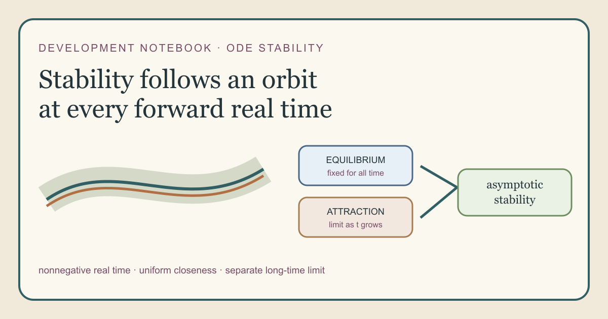
Stability and Attraction for ODE Flows in Lean

Begin with two flows

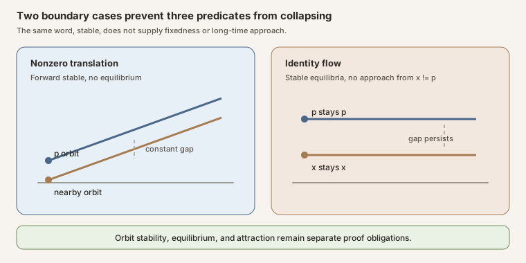
For a real constant \(c\), translation is the flow

\[ \Phi_c(t,x)=x+tc. \]

Two starts \(p\) and \(x\) keep the same separation:

\[ |\Phi_c(t,x)-\Phi_c(t,p)|=|x-p| \]

for every real \(t\). Translation is therefore forward stable at every reference point. If \(c\ne0\), no point is an equilibrium because \(\Phi_c(1,p)=p+c\ne p\). This checked counterexample refutes the universal claim that a forward-stable reference point must be fixed.

The identity flow gives the complementary boundary:

\[ \Phi_0(t,x)=x. \]

Every point is a Lyapunov-stable equilibrium, but an orbit starting at \(x\ne p\) does not converge to \(p\). Stability says that close starts remain close. Attraction says that an orbit approaches a specified target.

Parallel translation trajectories keep a constant gap despite having no equilibrium, while identity trajectories are stable equilibria but distinct starts do not approach one another. — FigureTwo boundary cases: nonzero translation exhibits orbit stability without equilibrium. The identity flow exhibits Lyapunov-stable equilibria without attraction of a distinct start. These examples separate predicates; they do not classify all stable or attracting flows.

The reference object and time domain

The input is Mathlib’s Flow ℝ X, not an existential family of ODE solutions. A flow already contains joint continuity, the time-zero identity, and the additive action law. The previous milestone explains why unique global integral curves require joint continuous dependence before they form this structured object.

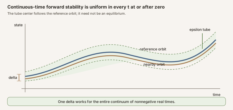
For forward stability, the family of maps is indexed by AddSubmonoid.nonneg ℝ, the subtype of real numbers satisfying (0\le t). The definition is

EquicontinuousAt (fun t : AddSubmonoid.nonneg ℝ ↦ ϕ t) p

This makes three choices visible:

time is continuous, not sampled at natural numbers;
the stability quantifier includes time zero and every nonnegative real time; and
one initial neighborhood must work uniformly for the entire family.

The negative-time maps still exist because the input is a real flow. They are not included in the forward-stability quantifier.

From uniform spaces to epsilon and delta

In a uniform space, EquicontinuousAt says that every requested entourage of the reference orbit has one initial neighborhood whose points stay inside that entourage for every family index.

In a pseudo-metric space, isForwardStableAt_iff_dist exposes the familiar form:

\[ \forall\varepsilon\gt0\;\exists\delta\gt0\;\forall x, d(x,p)\lt\delta\Longrightarrow \forall t\ge0,\quad d(\Phi(t,p),\Phi(t,x))\lt\varepsilon. \]

The radius \(\delta\) may depend on \(\varepsilon\), but not on the initial state \(x\) or the forward time \(t\). Separate continuity of each fixed-time map would allow a different radius for every \(t\); that weaker statement is not forward stability.

One delta interval at time zero maps into epsilon neighborhoods centered along every point of a continuous moving reference orbit for all nonnegative real times. — FigureUniform over forward time: one initial delta-neighborhood controls the full continuum of maps indexed by \(t\ge0\). The tube follows the reference orbit, so its center need not be stationary.

Equilibrium is a separate condition

IsEquilibrium ϕ p means

\[ \forall t\in\mathbb R,\quad \Phi(t,p)=p. \]

Because a real flow has inverse time maps, isEquilibrium_iff_nonneg proves that checking all nonnegative times is equivalent. This equivalence uses the flow law, not an unstated differential equation.

IsLyapunovStableEquilibrium ϕ p is the conjunction of equilibrium and forward stability. At an equilibrium, the moving center in the metric estimate reduces to \(p\):

\[ d(x,p)\lt\delta\Longrightarrow d(\Phi(t,x),p)\lt\varepsilon \quad\text{for every }t\ge0. \]

The theorem isLyapunovStableEquilibrium_iff_dist records that exact specialization.

Attraction uses a different limiting statement

The orbit from \(x\) is attracted to \(p\) when

\[ \Phi(t,x)\longrightarrow p\qquad(t\to+\infty). \]

In Lean this is Tendsto (fun t : ℝ ↦ ϕ t x) atTop (nhds p). The source then defines basinOfAttraction ϕ p as the set of starts satisfying that relation.

For a Hausdorff space, IsAttractedTo.isEquilibrium proves that any finite forward orbit limit of a continuous real flow is an equilibrium. Joint continuity enters through continuity of each fixed-time map. The action law then identifies the transported orbit with a time translate of the original orbit, and uniqueness of limits identifies the target with its image at every time.

That theorem does not turn attraction into Lyapunov stability. The definitions retain separate obligations:

Name	Required content
locally attracting equilibrium	equilibrium and a basin that is a neighborhood
globally attracting equilibrium	equilibrium and attraction of every start
asymptotically stable equilibrium	Lyapunov stability and a basin that is a neighborhood

The theorem isAsymptoticallyStableEquilibrium_iff unfolds the last row as Lyapunov stability plus local attraction.

Nonexpansive forward maps

If every forward-time map satisfies

\[ d(\Phi(t,x),\Phi(t,y))\le d(x,y), \]

then choosing \(\delta=\varepsilon\) proves forward stability at every point. The theorem isForwardStableAt_of_forall_lipschitzWith_one packages this criterion using Mathlib’s LipschitzWith 1 interface. Adding equilibrium gives isLyapunovStableEquilibrium_of_forall_lipschitzWith_one.

The identity and translation results are specializations of that criterion, not numerical simulations.

In Lean

One idea, three languages Read across, then read the syntax map

A human says

One initial neighborhood keeps every nearby orbit close to the reference orbit at all nonnegative real times.

On paper

\(\forall\varepsilon\gt0\;\exists\delta\gt0\;d(x,p)\lt\delta\Rightarrow\forall t\ge0,\ d(\Phi(t,p),\Phi(t,x))\lt\varepsilon.\)

In Lean

def IsForwardStableAt [UniformSpace X] (ϕ : Flow ℝ X) (p : X) : Prop := EquicontinuousAt (fun t : AddSubmonoid.nonneg ℝ ↦ ϕ t) p

Syntax map

Flow ℝ X supplies the jointly continuous real action. The subtype AddSubmonoid.nonneg ℝ carries a real time together with a proof that it is nonnegative. EquicontinuousAt chooses the source neighborhood before it quantifies over every such time.

One idea, three languages Read across, then read the syntax map

A human says

An asymptotically stable equilibrium is both Lyapunov stable and locally attracting.

On paper

\(\operatorname{AsympStable}(p)\iff\operatorname{LyapStable}(p)\land B(p)\in\mathcal N(p).\)

In Lean

theorem isAsymptoticallyStableEquilibrium_iff : IsAsymptoticallyStableEquilibrium ϕ p ↔ IsLyapunovStableEquilibrium ϕ p ∧ IsLocallyAttractingEquilibrium ϕ p

Syntax map

B(p) is basinOfAttraction ϕ p. Membership in nhds p says the basin contains some neighborhood of \(p\). The theorem is an exact interface identity, not a Lyapunov-function criterion.

Try it in the repository

import NonlinearDynamics.Deterministic.ODE.Stability

open NonlinearDynamics.Deterministic.ODE

#check IsForwardStableAt
#check IsEquilibrium
#check IsLyapunovStableEquilibrium
#check IsAttractedTo
#check basinOfAttraction
#check isForwardStableAt_iff_dist
#check IsAttractedTo.isEquilibrium
#check forwardStableAt_translationFlow_not_equilibrium
#check isAttractedTo_id_iff
#check isAsymptoticallyStableEquilibrium_iff

This is a full project check on macOS or Linux. It uses the repository’s pinned Lean and Mathlib dependencies; initial setup may require substantial disk space and build time.

Try it in the repository NonlinearDynamics/Deterministic/ODE/Stability.lean

The command checks the complete source with warnings treated as errors. Lean’s kernel checks the formal statements and proof terms; it does not certify that a chosen flow models a particular physical system.

Full project check, from the repository root

cd formalization
lake env lean -DwarningAsError=true NonlinearDynamics/Deterministic/ODE/Stability.lean

Resource note: this exact file uses the repository's pinned Lean and Mathlib dependencies. Initial project setup can require substantial disk space and build time. For a lightweight first step on macOS or Linux, use the page's standalone Lean-core or Std tutorial.

cd formalization
lake env lean -DwarningAsError=true \
  NonlinearDynamics/Deterministic/ODE/Stability.lean

Declaration map and nonclaims

Declaration	Role
`IsForwardStableAt`	equicontinuity of all nonnegative-time maps
`IsEquilibrium`	fixedness at every real time
`IsLyapunovStableEquilibrium`	equilibrium plus forward stability
`IsAttractedTo`	real-time convergence to a point at `atTop`
`basinOfAttraction`	starts attracted to one target
`IsLocallyAttractingEquilibrium`	equilibrium with a neighborhood basin
`IsGloballyAttractingEquilibrium`	equilibrium attracting every start
`IsAsymptoticallyStableEquilibrium`	Lyapunov stability plus local basin condition
`isForwardStableAt_iff`	entourage-and-neighborhood unfolding
`isForwardStableAt_iff_dist`	orbitwise epsilon-delta form
`isLyapunovStableEquilibrium_iff_dist`	equilibrium-centered metric form
`isEquilibrium_iff_nonneg`	forward-time equilibrium test
`isForwardStableAt_of_forall_lipschitzWith_one`	common nonexpansive criterion
`isLyapunovStableEquilibrium_of_forall_lipschitzWith_one`	nonexpansive equilibrium criterion
`isForwardStableAt_id`	identity-flow stability
`isLyapunovStableEquilibrium_id`	identity-flow Lyapunov stability
`translationFlow` and `translationFlow_apply`	constant-velocity example
`isForwardStableAt_translationFlow`	translation-orbit stability
`forwardStableAt_translationFlow_not_equilibrium`	stable non-equilibrium counterexample
`mem_basinOfAttraction`	basin membership unfolding
`isAttractedTo_iff_dist`	metric attraction form
`IsEquilibrium.isAttractedTo`	equilibrium attracts its own orbit
`IsAttractedTo.isEquilibrium`	Hausdorff flow limit is equilibrium
`isAttractedTo_id_iff`	identity-flow attraction boundary
`IsGloballyAttractingEquilibrium.isLocallyAttractingEquilibrium`	global-to-local implication
`isAsymptoticallyStableEquilibrium_iff`	stable-and-attracting decomposition

Not claimed: a Lyapunov-function theorem; exponential or input-to-state stability; stability of invariant sets; stable manifolds; robustness under perturbations of a vector field or flow; structural stability; stochastic stability of invariant laws or growth rates; or validation of a physical ODE.

References

N. P. Bhatia and G. P. Szegő, Dynamical Systems: Stability Theory and Applications, Lecture Notes in Mathematics 35, Springer, 1967, especially the metric-space stability development. Publisher record.
J. P. LaSalle, The Stability of Dynamical Systems, CBMS-NSF Regional Conference Series in Applied Mathematics 25, SIAM, 1976. Publisher record.
Mathlib contributors, Mathlib.Dynamics.Flow, version 4.32.0.
Mathlib contributors, Topology.UniformSpace.Equicontinuity and Topology.MetricSpace.Equicontinuity, version 4.32.0.

Discussion

This milestone makes stability a consumer of the structured flow layer. The definition does not reach backward into existential ODE solutions, and the proof that an orbit limit is an equilibrium uses exactly the two flow features it needs: continuity and the additive action law.

The interface also records the project-wide stability decision in a local, auditable form. Deterministic orbit stability controls nearby states under one fixed evolution. Structural stability would compare different evolutions. Stochastic stability would require a specified random object and a topology of perturbation, such as the separately selected upper-semicontinuity statement for integrated random-cocycle growth rates. Reusing one unqualified word for those different inputs and conclusions would erase the theorem’s content.