Start with three states
Let the state space be low, middle, and high, with
The orbit from high reaches low after two updates. The orbit from
middle reaches it after one, and the orbit from low is already constant.
All three states therefore lie in the basin of the fixed point low.
This finite example is stronger than a sample calculation because the three constructors exhaust the state type. It establishes the stated basin for this model, not for arbitrary maps.
Convergence defines the point basin
For a map \(f:X\to X\), define
\[ B_f(p)=\{x\in X:f^n(x)\to p\}. \]Membership is about the complete limiting tail. Visiting a neighborhood once does not suffice, and reaching \(p\) at one time does not suffice unless later iterates remain appropriately close.
def IsAttractedTo [TopologicalSpace X]\n (f : X → X) (x p : X) : Prop :=\n Tendsto (fun n : ℕ ↦ f^[n] x) atTop (𝓝 p)f^[n] is the n-fold function iterate. atTop represents arbitrarily late
natural-number times. 𝓝 p contains the neighborhoods of p. Tendsto
means every such neighborhood contains all sufficiently late iterates.In a pseudo-metric space, the same statement is
\[ d(f^n(x),p)\to0. \]The theorem isAttractedTo_iff_dist uses Mathlib’s
tendsto_iff_dist_tendsto_zero for this translation.
Local attraction is a neighborhood condition
The point \(p\) is a locally attracting fixed point when
\[ f(p)=p \quad\text{and}\quad B_f(p)\in\mathcal N(p). \]The filter statement says that the basin contains some neighborhood of \(p\). It does not say the basin is only local. The basin may extend far beyond the neighborhood used by the definition.
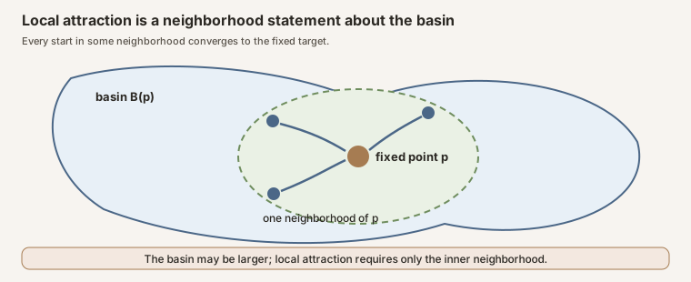
Global attraction quantifies over every initial state. The theorem
IsGloballyAttractingFixedPoint.isLocallyAttractingFixedPoint restricts that
universal statement to a neighborhood.
Attraction and stability answer different questions
Forward stability asks whether a nearby start remains close to the reference orbit at every time. Attraction asks whether the orbit approaches a target as time tends to infinity.
A transient can be large even when the eventual limit is \(p\). Conversely, two translated trajectories may stay a constant distance apart forever, so the reference orbit is stable without attracting the nearby orbit.
The project therefore defines
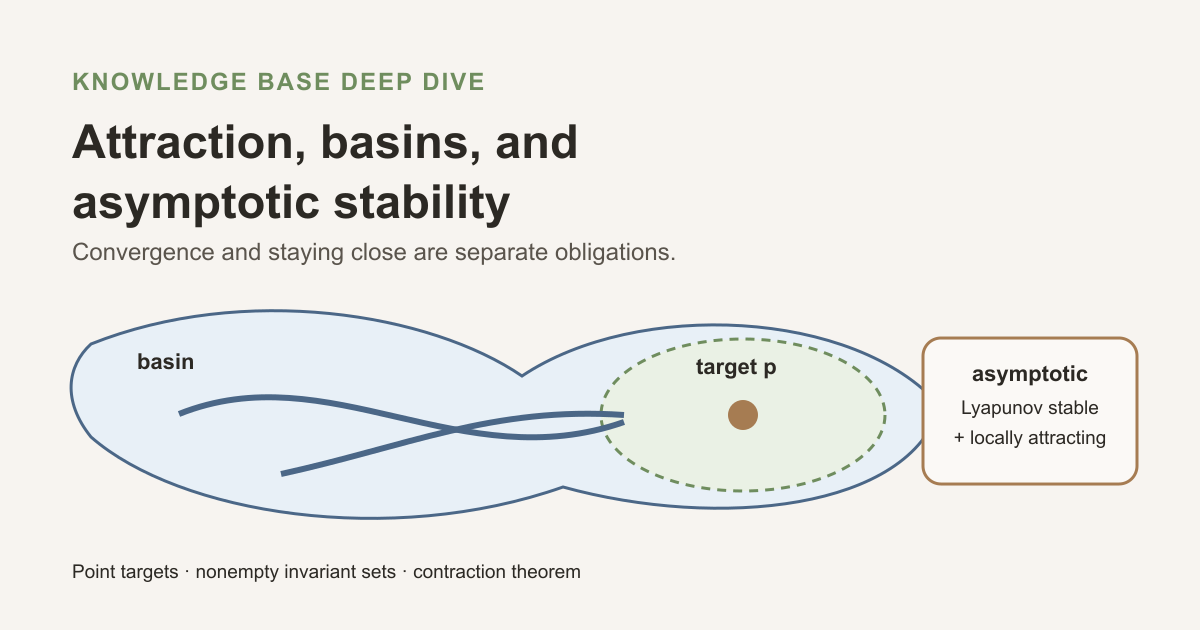
\[ \begin{aligned} \text{asymptotically stable fixed point} &= \text{Lyapunov-stable fixed point}\\ &\quad+\text{local attraction}. \end{aligned} \]The plus sign denotes conjunction, not numerical addition.
def IsAsymptoticallyStableFixedPoint [UniformSpace X]\n (f : X → X) (p : X) : Prop :=\n IsLyapunovStableFixedPoint f p ∧\n basinOfAttraction f p ∈ 𝓝 pIsLocallyAttractingFixedPoint.Why contractions are the clean test case
Suppose \(f\) has Lipschitz constant \(K\lt1\) on a nonempty complete metric space. Mathlib’s Banach fixed-point API constructs a unique fixed point and proves
\[ f^n(x)\to p \]for every \(x\). This gives a global basin. Since \(K\le1\), the same map is nonexpansive, and the preceding stability module proves forward stability. The two results together yield asymptotic stability.
The source reuses Mathlib’s theorem rather than encoding a second contraction proof. Completeness and nonemptiness remain visible because the constructed fixed point needs them.
Attraction to a set
For a nonempty set \(A\subseteq X\), the orbit from \(x\) is attracted to \(A\) when
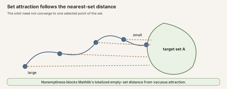
\[ \operatorname{dist}(f^n(x),A)\to0. \]The orbit need not converge to one selected point in \(A\). It may approach different parts of the set at different times.
def IsAttractedToSet [PseudoMetricSpace X]\n (f : X → X) (x : X) (A : Set X) : Prop :=\n A.Nonempty ∧\n Tendsto (fun n : ℕ ↦ Metric.infDist (f^[n] x) A)\n atTop (𝓝 0)Metric.infDist y A is the infimum distance from y to A. The explicit
A.Nonempty blocks the totalized identity Metric.infDist y ∅ = 0 from
turning the empty set into a universal target.A locally attracting set is also required to be forward invariant and to have its basin as a neighborhood of each point in the set. This milestone chooses forward inclusion \(f(A)\subseteq A\), not equality invariance.
For a singleton, Metric.infDist_singleton recovers the ordinary point
distance. Three checked bridge theorems identify orbit attraction, basins, and
local attraction for \(A=\{p\}\).
Standalone Lean tutorial
The file finite-basin.lean imports only Std. It defines the three-state
system, proves an eventual constant tail for every constructor, and evaluates
the first five states of the high orbit.
def reachesLow (x : State) : Prop :=
  ∃ N, ∀ n, N ≤ n → orbit x n = low

theorem every_state_reachesLow (x : State) : reachesLow x := by
  refine ⟨2, fun n hn => ?_⟩
  obtain ⟨k, rfl⟩ := Nat.exists_eq_add_of_le hn
  simpa [Nat.add_comm, Nat.add_left_comm, Nat.add_assoc] using
    orbit_after_two x k
The bundled file contains the complete definitions and supporting lemmas. Run it on macOS or Linux:
elan run leanprover/lean4:v4.32.0 lean \
  site/content/knowledge-base/deep-dives/attraction-basins-and-asymptotic-stability-in-discrete-time/finite-basin.lean
Try it in the repository
The exact source is a full project check using pinned Lean and Mathlib dependencies and may require substantial disk space or setup time:
import NonlinearDynamics.Deterministic.Discrete.Attraction

#check IsAttractedTo
#check basinOfAttraction
#check IsAsymptoticallyStableFixedPoint
#check isAttractedToSet_singleton_iff
NonlinearDynamics/Deterministic/Discrete/Attraction.lean; the command below
checks that complete module with the repository’s pinned environment.cd formalization
lake env lean -DwarningAsError=true NonlinearDynamics/Deterministic/Discrete/Attraction.leanResource note: this exact file uses the repository's
pinned Lean and Mathlib dependencies. Initial project setup can require
substantial disk space and build time. For a lightweight first step on
macOS or Linux, use the page's standalone Lean-core or Std
tutorial.
Boundaries
This interface does not define uniform attraction of bounded sets, compact global attractors, equality invariance, Hausdorff convergence, invariant-set Lyapunov stability, periodic attractors, attraction rates, robustness under map perturbations, or stable manifolds.
Continue to Lyapunov Functions and the Direct Method in Discrete Time for a scalar-certificate route that keeps stability and attraction as separate conclusions.
References
- J. P. LaSalle, “Difference Equations. Discrete Semidynamical Systems,” in The Stability of Dynamical Systems, SIAM CBMS 25 (1976), pages 1–25, DOI 10.1137/1.9781611970432.ch1.
- Jack K. Hale, Asymptotic Behavior of Dissipative Systems, AMS Surveys and Monographs 25 (1988), Chapter 2, DOI 10.1090/surv/025.
- Mathlib 4.32.0, pinned revision
81a5d257, source modulesTopology.MetricSpace.Contracting,Topology.MetricSpace.HausdorffDistance, andDynamics.FixedPoints.Topology.