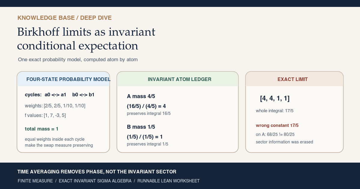
Start with four states and one probability measure
Take the finite state space
\[ \Omega=\{a_0,a_1,b_0,b_1\}. \]Let \(T\) swap \(a_0\) with \(a_1\) and swap \(b_0\) with \(b_1\). Give the four points probabilities
\[ \mu(a_0)=\mu(a_1)=\frac25, \qquad \mu(b_0)=\mu(b_1)=\frac1{10}. \]The normalization is exact:
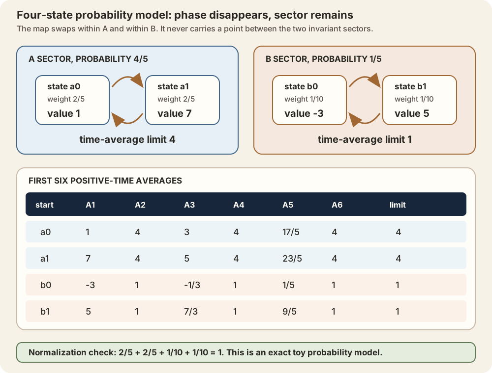
\[ \frac25+\frac25+\frac1{10}+\frac1{10}=1. \]Equal weights within each two-cycle make \(T\) measure preserving. Choose the observable
\[ f(a_0)=1,\qquad f(a_1)=7,\qquad f(b_0)=-3,\qquad f(b_1)=5. \]For positive \(n\), the Birkhoff average is
\[ A_nf(\omega) {} = \frac1n\sum_{j=0}^{n-1}f\bigl(T^j\omega\bigr). \]Starting at \(a_0\), the first six averages are
\[ 1,\quad4,\quad3,\quad4,\quad\frac{17}{5},\quad4. \]Starting at \(a_1\), they are
\[ 7,\quad4,\quad5,\quad4,\quad\frac{23}{5},\quad4. \]Every even average in the \(a\)-cycle is \(4\), and the odd error has magnitude \(3/n\). Both \(a\)-states therefore have limit \(4\).
The corresponding rows for \(b_0\) and \(b_1\) are
\[ \begin{aligned} b_0 &: -3,\ 1,\ -\frac13,\ 1,\ \frac15,\ 1,\\ b_1 &: 5,\ 1,\ \frac73,\ 1,\ \frac95,\ 1. \end{aligned} \]Every even average in the \(b\)-cycle is \(1\), and both \(b\)-states have limit \(1\).
Enumerate the invariant information
A set \(s\subseteq\Omega\) is exactly invariant when \(T^{-1}s=s\). In this model, an invariant set contains both members of a two-cycle or neither. Therefore the exact invariant sigma-algebra is
\[ \mathcal I_T {} = \{\varnothing,\ A,\ B,\ \Omega\}, \]where
\[ A=\{a_0,a_1\}, \qquad B=\{b_0,b_1\}. \]Its two nonempty atoms have masses
\[ \mu(A)=\frac45, \qquad \mu(B)=\frac15. \]An \(\mathcal I_T\)-measurable real function must be constant on \(A\) and constant on \(B\). Write those two values as \(c_A\) and \(c_B\).
Compute conditional expectation atom by atom
Conditional expectation onto \(\mathcal I_T\) must preserve the integral on each invariant atom. On \(A\),
\[ \int_A f\,d\mu {} = \frac25(1)+\frac25(7) {} = \frac{16}{5}. \]Thus
\[ \frac45c_A=\frac{16}{5}, \qquad c_A=\frac{16/5}{4/5}=4. \]On \(B\),
\[ \int_B f\,d\mu {} = \frac1{10}(-3)+\frac1{10}(5) {} = \frac15. \]Thus
\[ \frac15c_B=\frac15, \qquad c_B=\frac{1/5}{1/5}=1. \]The conditional expectation is therefore the exact vector
\[ \mathbb E_\mu[f\mid\mathcal I_T] {} = (4,4,1,1). \]It agrees point by point with the two Birkhoff limits. Its whole-space integral is also preserved:
\[ \int_\Omega f\,d\mu {} = \frac{17}{5} {} = \int_\Omega\mathbb E_\mu[f\mid\mathcal I_T]\,d\mu. \]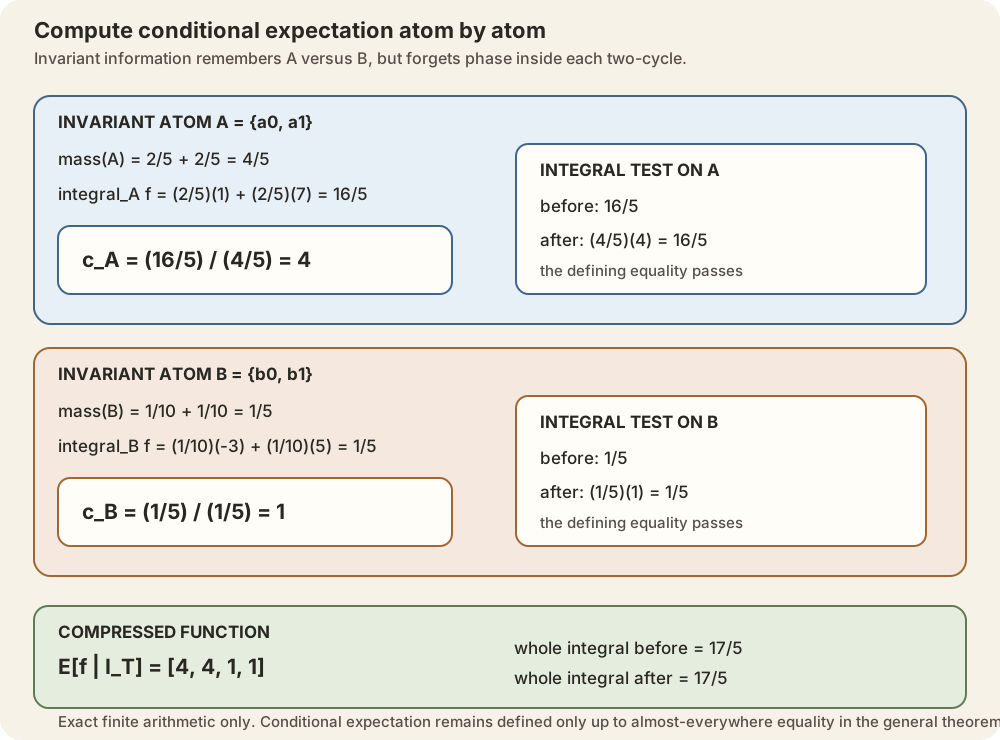
Audit four nearby wrong turns
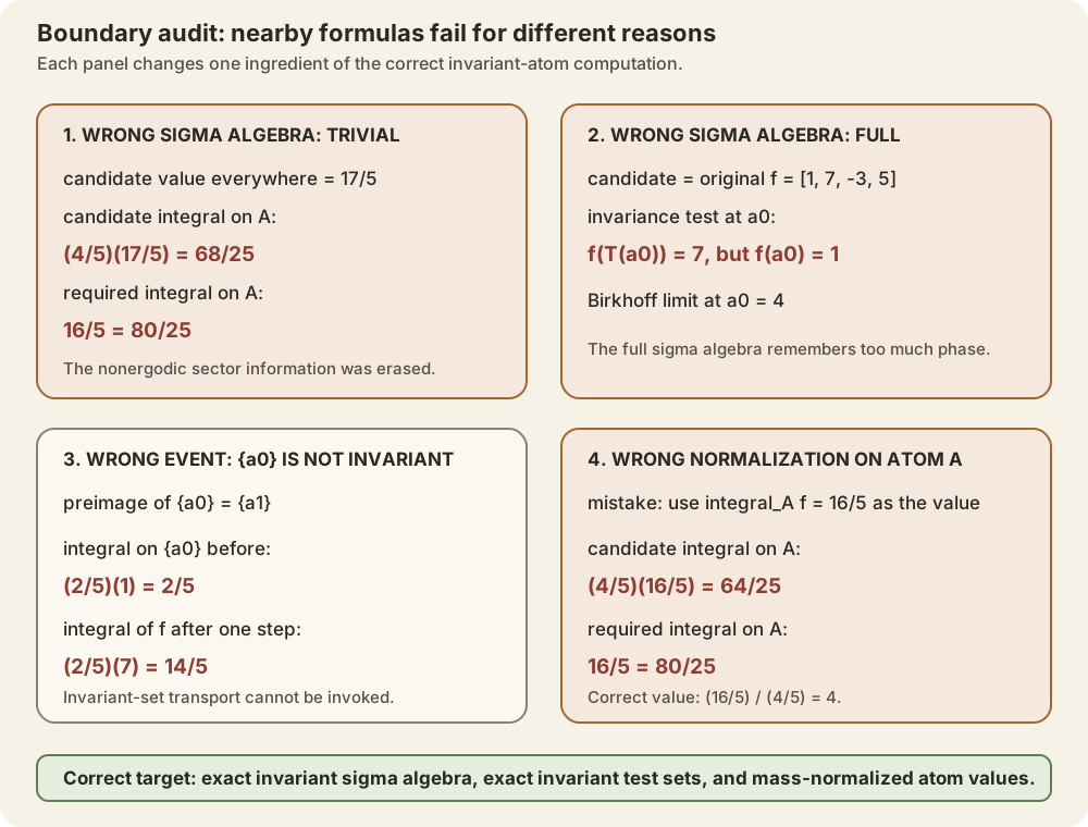
Four nearby substitutions give incorrect answers.
- Sigma-algebra too small. Conditioning on the trivial sigma-algebra gives the global constant \(17/5\). Its integral on \(A\) is \((4/5)(17/5)=68/25\), but the required value is \(16/5=80/25\).
- Sigma-algebra too large. Conditioning on the full sigma-algebra returns \(f\), which is not invariant because \(f(Ta_0)=7\ne1=f(a_0)\).
- Wrong test set. The singleton \(\{a_0\}\) is measurable but not invariant: \(T^{-1}\{a_0\}=\{a_1\}\). Its original integral is \(2/5\), while the integral of \(f\circ T\) over it is \(14/5\). The invariant-set transport theorem does not apply.
- Wrong normalization. Using the raw atom integral \(16/5\) as the value on \(A\) forgets to divide by \(\mu(A)=4/5\). That candidate integrates to \((4/5)(16/5)=64/25\), not \(16/5=80/25\).
From the model to the finite-measure theorem
An orbit can forget its starting phase without forgetting which invariant part of the state space it inhabits. That is the central idea of the pointwise ergodic theorem with limit identification.
Let \(\Omega\) now be any measurable state space, let \(\mu\) be any finite measure, let \(T:\Omega\to\Omega\) preserve \(\mu\), and let \(f:\Omega\to\mathbb R\) be integrable. RMT-26 established that the Birkhoff averages converge for almost every \(\omega\). RMT-27 identifies the limit:
\[ A_n f(\omega) \longrightarrow \mathbb E_\mu\!\left[f\mid\mathcal I_T\right](\omega) \quad\text{for }\mu\text{-almost every }\omega. \]Here \(\mathcal I_T\) is the sigma-algebra of measurable sets satisfying the literal equation \(T^{-1}s=s\). The right side is the unique integrable \(\mathcal I_T\)-measurable function having the same integral as \(f\) on every set in \(\mathcal I_T\), up to almost-everywhere equality.
Identification is not merely a prettier name for an existing pointwise limit. Pointwise convergence does not permit passing integrals to the limit. Invariance almost everywhere is not the same object as measurability for Mathlib’s exact invariant sigma-algebra. A possibly noninjective transformation prevents a careless change-of-variables argument. An integrable Lean function may be only almost everywhere strongly measurable, while the invariant-space interface initially wants a literal strongly measurable representative.
The finite example used a probability measure to make the arithmetic familiar. The checked theorem needs only finite total mass; it does not assume probability normalization, ergodicity, injectivity, surjectivity, or invertibility. Its declaration-complete implementation diary is Identifying the Finite-Measure Birkhoff Limit in Lean. The reusable concepts have focused entries on the invariant sigma-algebra, conditional expectation, and uniform integrability.
Choose a route up
| Route | Begin | Destination |
|---|---|---|
| Concrete route | Start with four states and one probability measure | Compute both invariant-atom limits exactly |
| Information route | Invariant sets are the information time cannot erase | Understand the target sigma-algebra |
| Measure route | Why almost-everywhere convergence is not enough | Discover the need for uniform integrability |
| Proof route | The five bridges | Follow the full identification architecture |
| Lean route | The checked declaration map | Match all 18 public declarations to their jobs |
| Boundary route | Five compiled boundary probes | Audit every absent hypothesis |
| History route | Source ledger and theorem alignment | Separate historical statements from the Lean theorem |
| Practice route | Thirty solved exercises | Rebuild the chapter independently |
Learning objectives
By the summit, a reader should be able to:
- compute Birkhoff averages on a finite orbit decomposition;
- define the exact invariant sigma-algebra \(\mathcal I_T\);
- distinguish exact invariance from invariance modulo a null set;
- characterize conditional expectation by measurability and set integrals;
- explain why a nonergodic limit need not be constant;
- explain why almost-everywhere convergence alone cannot pass integrals;
- recognize a sequence that is not uniformly integrable;
- use identical distribution to obtain uniform integrability of orbit translates;
- use Cesaro stability to control all Birkhoff averages;
- state the finite-measure Vitali upgrade from pointwise to \(L^1\) convergence;
- transport integrals over invariant sets without assuming an embedding;
- explain why conditional-expectation uniqueness identifies the limit;
- distinguish a total pointwise representative from an almost-everywhere class;
- explain why the fallback branch of that representative must also be invariant;
- track strong measurability through the exact invariant-space interface;
- transport the theorem across almost-everywhere equal observables;
- read every public declaration and every boundary probe in the RMT-27 module;
- state exactly which assumptions the final theorem does not use; and
- run the tiny
Stdworksheet and distinguish it from the full project/Mathlib check.
Common setup and three kinds of equality
A measurable space specifies which subsets of \(\Omega\) may be assigned measure. A measure \(\mu\) assigns a nonnegative extended real size to those sets, with countable additivity. The assumption that \(\mu\) is finite means
\[ \mu(\Omega)\lt\infty. \]It does not mean \(\mu(\Omega)=1\). A finite measure can have total mass zero, five, or any other finite nonnegative value.
A map \(T:\Omega\to\Omega\) is measure preserving when it is measurable and its pushforward leaves the measure unchanged. In set language,
\[ \mu\bigl(T^{-1}s\bigr)=\mu(s) \]for every measurable \(s\). This equation does not imply that \(T\) is injective or surjective as a function.
Three kinds of equality recur throughout the proof.
| Equality | Meaning | Why it matters |
|---|---|---|
| \(u=v\) | literal equality of functions or sets | Needed by exact invariant interfaces |
| \(u=v\) almost everywhere | the disagreement set is null | Natural equality for integration and \(L^1\) |
| equality in \(L^1(\mu)\) | equality of almost-everywhere equivalence classes | Natural equality in the Banach space |
Collapsing these layers is one of the fastest ways to create a plausible but incorrect ergodic proof. The formal types require each transition to be explicit.
The repository’s Birkhoff average is totalized at horizon zero. The sum over an empty range is zero and the real inverse of zero is zero, so
\[ A_0f(\omega)=0. \]This convention makes \(n\mapsto A_nf(\omega)\) a sequence indexed by all natural numbers. It does not change its limit, which depends only on the tail. Any identity claimed for every horizon must nevertheless respect this zero term. That is why the invariant-set integral identity for averages is stated only when \(n\ne0\), while the uniform-integrability statement covers the complete totalized sequence.
Invariant sets are the information time cannot erase
A measurable set \(s\subseteq\Omega\) is exactly invariant under \(T\) if
\[ T^{-1}s=s. \]The exactly invariant measurable sets form a sigma-algebra, denoted here by
\(\mathcal I_T\). Mathlib constructs it as
MeasurableSpace.invariants T. A sigma-algebra can be read as an information
boundary: if one is told only which sets in that sigma-algebra contain the
current state, then one has exactly the distinctions that the sigma-algebra
can express.
In the four-point model, an invariant set must contain a whole two-cycle or none of it. Therefore
\[ \mathcal I_T {} = \bigl\{\varnothing, \{a_0,a_1\}, \{b_0,b_1\}, \Omega\bigr\}. \]The individual phase labels \(a_0\) versus \(a_1\) are not invariant information: one application of \(T\) swaps them. The sector label \(a\) versus \(b\) is invariant information: no iterate crosses sectors. Long-time averaging removes phase but retains sector.
An exactly invariant real function \(g\) satisfies
\[ g(T\omega)=g(\omega) \]at every point. Under the ambient measurability hypothesis, this is equivalent
to measurability of \(g\) from MeasurableSpace.invariants T into the Borel
real line. In the finite model, that says precisely that \(g\) is constant on
each two-cycle. It need not take the same value on distinct cycles.
This gives a useful hierarchy:
- ordinary measurability permits \(g\) to distinguish any measurable state;
- invariant measurability permits only distinctions stable under \(T\);
- ergodicity says invariant measurable distinctions are trivial modulo null sets; and
- probability normalization merely fixes total mass at one and supplies no ergodicity by itself.
Exact invariance and invariance modulo null sets
There are two nearby invariant sigma-algebras in the literature.
- Exact invariance requires \(T^{-1}s=s\) as literal sets.
- Modulo-null invariance requires the symmetric difference \(T^{-1}s\mathbin{\triangle}s\) to have measure zero.
They encode the same information only after an appropriate completion and an almost-everywhere interpretation. They are not definitionally the same object. Hess, Seri, and Choirat explicitly distinguish exact invariant sets from almost-sure invariant sets and state that the latter form the completion of the former in their probability setting. Chacon’s identification is also formulated through an invariant field completed modulo null sets. RMT-27 uses Mathlib’s exact sigma-algebra and builds a literal invariant representative before passing to almost-everywhere equality.
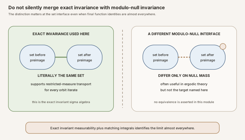
The distinction is visible on the boundary probe with \(\Omega=\{\mathsf{false},\mathsf{true}\}\), \(T\) the constant map to \(\mathsf{false}\), and \(\mu=\delta_{\mathsf{false}}\). The only exact invariant sets are \(\varnothing\) and \(\Omega\). Yet the singleton \(\{\mathsf{true}\}\) is equal modulo \(\mu\)-null sets to \(\varnothing\), and \(\{\mathsf{false}\}\) is equal modulo null sets to \(\Omega\). A theorem about the completed invariant field cannot be passed directly to an interface expecting literal preimage equality.
There is a second subtlety involving iterates. Every \(T\)-invariant set is
invariant under \(T^i\), but the reverse can fail. In the four-point swap,
\(T^2\) is the identity, so every set is \(T^2\)-invariant even though only
unions of the two cycles are \(T\)-invariant. The Lean proof uses
MeasurableSpace.le_invariants_iterate T i only in the safe direction.
Conditional expectation as the best invariant summary
Let \(\mathcal B\) be a sub-sigma-algebra of the ambient measurable space. For an integrable real function \(f\), a conditional expectation \(\mathbb E_\mu[f\mid\mathcal B]\) is characterized, up to almost-everywhere equality, by three requirements:
- it is measurable with respect to \(\mathcal B\);
- it is integrable; and
- for every \(s\in\mathcal B\),
This is an information-preserving compression. The conditional expectation forgets distinctions unavailable to \(\mathcal B\), while preserving all integrals that can be tested using \(\mathcal B\)-measurable events.
In the opening probability model, \(\mathcal B=\mathcal I_T\) has atoms \(A\) and \(B\). The computation \(c_A=4\), \(c_B=1\) is exactly this characterization on a finite atomic space. The wrong-target ledger shows why one cannot replace \(\mathcal I_T\) by either the trivial or full sigma-algebra.
The defining integral identity works for every finite measure, including a nonprobability measure. Atomwise division was available in the example because both invariant atoms had positive mass; it is an explanatory computation, not the definition used by the general theorem. On a positive-mass ergodic system, a later corollary could prove that the conditional expectation is constant and then identify that constant as
\[ \frac{1}{\mu(\Omega)}\int_\Omega f\,d\mu. \]That is not the RMT-27 theorem. Its general target remains the possibly nonconstant conditional expectation onto \(\mathcal I_T\). The zero measure also warns that division by \(\mu(\Omega)\) requires a separate positivity assumption.
The five bridges
RMT-26 supplies almost-everywhere convergence to some real limit at almost every point. The target formula requires five logically distinct bridges.
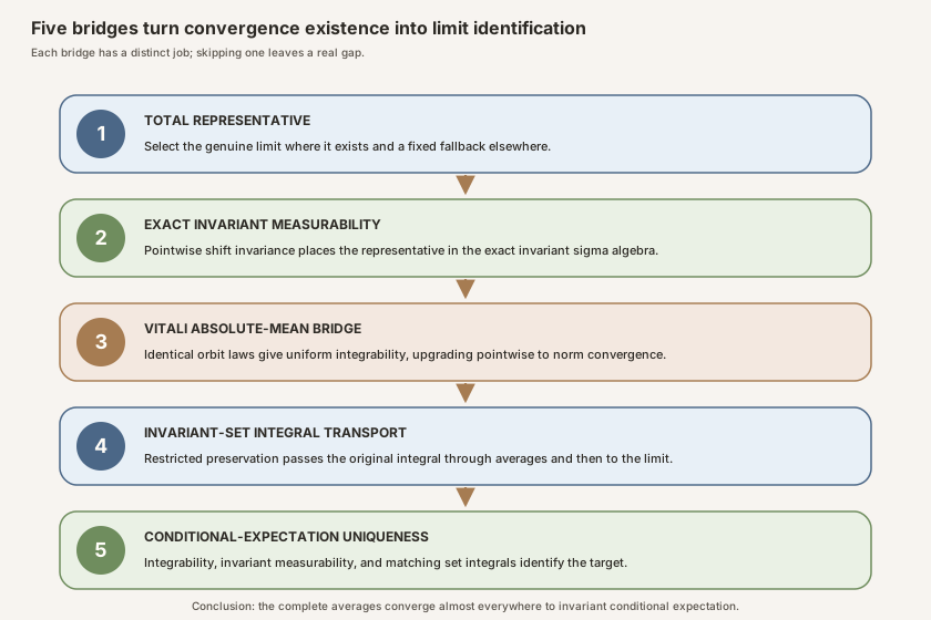
limUnder to choose one total representative. Bridge two proves literal invariance and exact-invariant measurability. Bridge three combines identical distributions, uniform integrability, and the finite-measure Vitali theorem to obtain \(L^1\) convergence. Bridge four transports each positive-time integral on an invariant set through a restricted measure. Bridge five applies the set-integral characterization of conditional expectation. Each bridge has a separate checked declaration; pointwise convergence alone skips bridges three through five.Bridge 1: choose one total limit
An almost-everywhere statement of the form
\[ \forall^{\mu}\omega, \quad \exists c, \quad A_nf(\omega)\to c \]does not by itself provide a globally defined function \(\omega\mapsto c\).
In Lean: choose one total representative
birkhoffLimit T f ωbirkhoffLimitis a total function, not a partially defined limit.Tis the base transformation andfis the observable.ωis the starting point.- The source unfolds the name to
limUnder atTop (fun n ↦ birkhoffAverage ℝ T f n ω). atTopsends the natural horizon to infinity.- No measurable-space, measure, integrability, or convergence premise is needed merely to define this representative.
At points where the sequence converges, Filter.limUnder
returns its unique limit. At divergent points, it returns the canonical value
provided by the nonempty real type. This fallback is not a mathematical claim
about a divergent sequence. It makes the representative total so that Lean
can discuss its measurability and invariance everywhere.
The construction is deliberately single and deterministic. Choosing an unrelated existential witness separately at each convergent point would make measurability hard to recover and would leave the divergent branch undefined.
Bridge 2: prove literal invariance and invariant measurability
The finite-prefix shift relation says that \(A_nf(T\omega)\) and \(A_nf(\omega)\) differ by endpoint terms divided by \(n\). Consequently, convergence at \(\omega\) is equivalent to convergence at \(T\omega\), and when convergence occurs the two limits are equal.
The fallback branch needs equal care. If the averages diverge at \(\omega\),
the reverse shift theorem shows that they diverge at \(T\omega\) too. Both
limUnder calls therefore use the same fallback. The module obtains the
pointwise equation
for every \(\omega\), not merely almost every \(\omega\).
In Lean: enter the exact invariant sigma-algebra
measurable_birkhoffLimit_invariants hT hfhT : Measurable Tsupplies ordinary measurability of the dynamics.hf : StronglyMeasurable fis the literal representative-level premise.Measurable[MeasurableSpace.invariants T]changes the domain sigma-algebra to the exact invariant one.birkhoffLimit_apply_base T f ωsupplies the pointwise equationbirkhoffLimit T f (T ω) = birkhoffLimit T f ω.MeasurableSpace.measurable_invariants_domcombines ambient measurability with that literal invariance.- The final identification is almost everywhere, but this intermediate invariance equation is exact.
For a strongly measurable \(f\) and measurable \(T\), every finite Birkhoff
average is strongly measurable. Mathlib’s StronglyMeasurable.limUnder
passes that property to the chosen limit. Ambient strong measurability plus
literal invariance then yields measurability with domain sigma-algebra
MeasurableSpace.invariants T.
Bridge 3: upgrade pointwise convergence to \(L^1\)
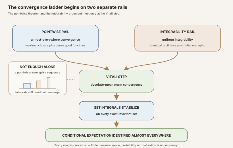
Almost-everywhere convergence does not generally preserve integrals. RMT-27 proves that all orbit translates \(f\circ T^i\) have the same distribution as \(f\). An integrable identically distributed family is uniformly integrable in \(L^1\). Cesaro averaging preserves uniform integrability, so the complete sequence \(A_nf\), including \(A_0f=0\), is uniformly integrable.
The finite-measure Vitali theorem then combines uniform integrability and almost-everywhere convergence to show
\[ \lVert A_nf-\operatorname{birkhoffLimit}(T,f)\rVert_1 \longrightarrow 0. \]This simultaneously proves that the chosen limit is integrable.
Bridge 4: preserve integrals on invariant sets
Fix an exactly \(T\)-invariant measurable set \(s\). It is invariant under every iterate \(T^i\). Because \(T^i\) preserves \(\mu\), its restriction transports the restricted measure \(\mu|_s\) to itself. Therefore
\[ \int_s f\bigl(T^i\omega\bigr)\,d\mu(\omega) {} = \int_s f(\omega)\,d\mu(\omega). \]Average these identities over \(i=0,\ldots,n-1\) for \(n\ne0\) to obtain
\[ \int_s A_nf\,d\mu {} = \int_s f\,d\mu. \]In Lean: preserve the integral on an exact invariant event
setIntegral_birkhoffAverage_eq hT hf hs hnhs : MeasurableSet[MeasurableSpace.invariants T] spackages ambient measurability and exact preimage invariance.hn : n ≠ 0excludes the totalized horizon-zero average.setIntegral_orbit_iterate_eqproves the equality for every individual orbit translate.MeasurePreserving.restrict_preimagetransports the restricted measure without injectivity or surjectivity.integral_finsetSumandintegral_smulaverage the termwise identities.- The conclusion concerns one exact invariant event, not an arbitrary measurable set.
Finally, \(L^1\) convergence lets the left side pass to the chosen limit.
Bridge 5: invoke conditional-expectation uniqueness
The chosen limit is integrable and measurable for \(\mathcal I_T\). Its integral on every \(s\in\mathcal I_T\) equals the integral of \(f\). These are exactly the hypotheses of Mathlib’s conditional-expectation uniqueness theorem. Hence
\[ \operatorname{birkhoffLimit}(T,f) {} = \mathbb E_\mu[f\mid\mathcal I_T] \quad\mu\text{-almost everywhere}. \]Combining this equality with convergence to birkhoffLimit gives the final
pointwise theorem.
In Lean: identify the chosen limit
birkhoffLimit_ae_eq_condExp hT hfhT : MeasurePreserving T μ μsupplies measurability, preservation of orbit distributions, and restricted-measure transport.hf : Integrable f μsupplies an \(L^1\) observable; it need not be literally strongly measurable.birkhoffLimit_ae_eq_condExp_of_stronglyMeasurableis the private helper that first proves the identification for a strong representative.birkhoffLimit_ae_eq_of_ae_eqtransports the chosen limit across almost-everywhere equal representatives.condExp_congr_aeperforms the corresponding transport for conditional expectation.=ᵐ[μ]means equality outside a \(\mu\)-null set, not pointwise equality at every state.
Why almost-everywhere convergence is not enough
On \((0,1)\) with Lebesgue measure, define
\[ h_n(x)=n\,\mathbf 1_{(0,1/n)}(x). \]Every \(x\in(0,1)\) is positive, so eventually \(x\notin(0,1/n)\) and \(h_n(x)\to0\). The convergence is pointwise everywhere. Nevertheless,
\[ \int_0^1 h_n(x)\,dx=1 \qquad\text{and}\qquad \lVert h_n\rVert_1=1 \]for every \(n\). The mass concentrates into an increasingly narrow and high spike. Pointwise convergence sees each fixed point eventually escape the spike; integration sees one unit of mass forever.
The family is not uniformly integrable. For any cutoff \(K\gt0\), choose \(n\gt K\). Then the whole support lies where \(|h_n|\gt K\), and
\[ \int_{\{|h_n|\gt K\}} |h_n|\,d\mu=1. \]Uniform integrability rules out this escape mechanism uniformly across the sequence. In one standard operational form, a family \(\{u_n\}\) is uniformly integrable when its large-value tails satisfy
\[ \lim_{K\to\infty} \sup_n \int_{\{|u_n|\gt K\}}|u_n|\,d\mu {} =0, \]together with the measurability and integrability structure used by the chosen formal definition. The abbreviation UI will refer to uniform integrability below.
Identical distributions control orbit tails
For a measure-preserving \(T\), each iterate \(T^i\) also preserves \(\mu\). Therefore \(f\circ T^i\) and \(f\) have the same pushforward measure on \(\mathbb R\). In probability language, they are identically distributed. This statement needs no independence. Consecutive orbit readings are usually highly dependent.
Identical distribution means every orbit translate has the same tail profile. If \(f\) is integrable, the family
\[ \bigl\{f\circ T^i:i\in\mathbb N\bigr\} \]is uniformly integrable. Mathlib packages this through
MemLp.uniformIntegrable_of_identDistrib. The module supplies the iterate
\(i=0\) as the reference member and proves IdentDistrib for every other
iterate.
The Birkhoff averages are Cesaro means of this family. Convex averaging
cannot manufacture a new uniformly large tail from a uniformly integrable
family. Pinned Mathlib exposes this fact as uniformIntegrable_average.
RMT-27 then reconciles Mathlib’s abstract average with the repository’s
pointwise birkhoffAverage definition.
There is an important separation of roles:
- measure preservation supplies identical distribution;
- integrability of one observable supplies the \(L^1\) reference member;
- finite measure is used by the selected Vitali theorem and associated integrability interface;
- no independence, mixing, or ergodicity is used.
In Lean: control every average with uniform integrability
uniformIntegrable_birkhoffAverage hT hf[IsFiniteMeasure μ]is the finite-total-mass instance used by this selected interface.hT : MeasurePreserving T μ μgivesidentDistrib_orbit_iterate hT hf.aemeasurable ifor every \(i\).hf : Integrable f μsupplies the \(L^1\) reference member.uniformIntegrable_orbit_iteratecontrols the untranslated family.uniformIntegrable_averagepasses control through finite Cesaro averages.- The horizon-zero average is the zero function and remains part of the uniformly integrable sequence.
- No independence or ergodicity premise occurs.
Vitali closes the convergence gap
The finite-measure Vitali convergence theorem says, in the form used here, that a uniformly integrable sequence which converges almost everywhere to a measurable limit converges to that limit in \(L^1\). The RMT-27 sequence is \(u_n=A_nf\), and RMT-26 supplies its almost-everywhere convergence to the chosen total representative.
The Lean conclusion is written with the extended \(L^p\) norm at exponent one:
\[ \operatorname{eLpNorm} \bigl(A_nf-\operatorname{birkhoffLimit}(T,f),1,\mu\bigr) \longrightarrow0. \]In Lean: upgrade to \(L^1\) convergence
tendsto_L1_birkhoffAverage_birkhoffLimit hT hf- The result is a
Tendstostatement indexed by natural horizons atatTop. eLpNorm (...) 1 μis Mathlib’s extended \(L^p\) norm at exponent one.birkhoffAverage ℝ T f n - birkhoffLimit T fis the pointwise difference.tendsto_Lp_finite_of_tendsto_aeis the finite-measure Vitali bridge.uniformIntegrable_birkhoffAverage hT hfsupplies the tail control.ae_tendsto_birkhoffAverage_birkhoffLimit hT hfsupplies the pointwise convergence rail.- This theorem also consumes integrability of the chosen endpoint; pointwise convergence alone does not prove the conclusion.
At exponent one and under the established measurability and integrability hypotheses, this is the formal \(L^1\)-convergence statement needed by the set-integral continuity theorem.
The same uniform-integrability theorem also proves that the pointwise limit
is integrable. This matters twice. First, conditional expectation is an
integrable object. Second, the tendsto_setIntegral_of_L1' interface requires
the limit’s almost-everywhere strong measurability and the approximants'
integrability.
Restricted-measure transport avoids false invertibility
The tempting informal line
\[ \int_s f\circ T^i\,d\mu {} = \int_{T^i(s)}f\,d\mu \]is dangerous. It resembles a substitution theorem that may require injectivity, an inverse, or a measurable embedding. None is available in the general RMT-27 theorem.
Instead, begin with the restricted measure \(\mu|_s\). If \(s\) is exactly invariant under \(T^i\), then
\[ (T^i)^{-1}s=s. \]MeasurePreserving.restrict_preimage proves that \(T^i\) maps the measure
restricted to its preimage back to the target restricted measure. After the
exact invariant equation rewrites the preimage, this becomes
Now the ordinary integral-under-a-map theorem applies to the restricted measure. It transports \(f\circ T^i\) without claiming that \(T^i\) embeds the underlying space.
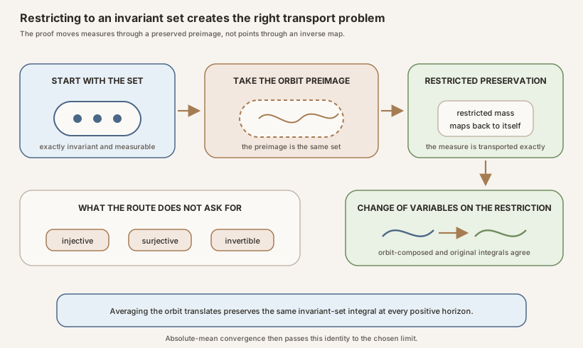
Once every orbit term has the same integral on \(s\), finite linearity gives the average identity for positive horizons. \(L^1\) convergence then gives
\[ \int_s \operatorname{birkhoffLimit}(T,f)\,d\mu {} = \int_s f\,d\mu. \]The proof first establishes this for exact invariant sets because those are the measurable sets of the target sigma-algebra. Almost-everywhere uniqueness then places the result naturally in the measure-theoretic quotient world.
Strong representatives and transport back
Lean’s Integrable f μ provides almost-everywhere strong measurability, not
necessarily literal StronglyMeasurable f. The construction of exact
invariant measurability is cleanest for a literal strongly measurable
function. The final theorem must still accept every integrable observable.
The module therefore uses a two-stage representative strategy.
- For a strongly measurable \(f\), prove the whole identification argument, ending in a private helper.
- For arbitrary integrable \(f\), choose the standard strongly measurable
representative \(f'\) supplied by
hf.aestronglyMeasurable.mk f. - Prove \(f=f'\) almost everywhere.
- Transport Birkhoff limits across that equality using quasi-measure preservation.
- Transport conditional expectations with
condExp_congr_ae.
The new public declaration birkhoffLimit_ae_eq_of_ae_eq is the central
transport lemma. If \(f=g\) almost everywhere and \(T\) is quasi-measure
preserving, then every finite orbit average agrees almost everywhere. Taking
a countable intersection over all horizons yields one conull set on which
the entire two sequences are pointwise equal. Their limUnder values are
therefore equal on that set.
This lemma deliberately assumes only quasi-measure preservation, the property needed to pull null sets backward through iterates. The final theorem has the stronger measure-preserving hypothesis for the distributional and integral steps.
Conditional-expectation uniqueness is the summit
Mathlib’s ae_eq_condExp_of_forall_setIntegral_eq is an identification
principle. In the RMT-27 application, its candidate function is
birkhoffLimit T f, its target sub-sigma-algebra is
MeasurableSpace.invariants T, and its original function is \(f\).
The proof discharges three substantive obligations:
- integrability of the candidate on every invariant measurable set;
- equality of candidate and original set integrals on every such set; and
- almost-everywhere strong measurability of the candidate for the invariant sigma-algebra.
The order matters. Conditional expectation is not defined as “whatever the Birkhoff averages approach.” It is defined independently by its information and integral properties. The proof shows that the dynamical limit satisfies that independent characterization.
The final pointwise statement follows by intersecting two conull events:
- the Birkhoff averages tend to
birkhoffLimit T f; and birkhoffLimit T fequals the conditional expectation.
At a point in their intersection, rewriting the target of the first limit by the second equality completes the theorem.
The checked declaration map
The canonical module currently exposes 18 public declarations. The private strong-representative helper is intentionally not counted. Every public name has a distinct proof role.
| Number | Public declaration | Contract and role |
|---|---|---|
| 1 | birkhoffLimit | Defines one total real representative with limUnder, including a fallback at divergent points. |
| 2 | tendsto_birkhoffAverage_birkhoffLimit_of_exists | Turns existence of any finite limit at one point into convergence to the chosen representative. |
| 3 | tendsto_birkhoffAverage_birkhoffLimit_of_mem | Specializes the previous theorem to membership in birkhoffConvergenceSet. |
| 4 | birkhoffLimit_apply_base | Proves literal pointwise invariance under one application of \(T\), including the divergent fallback branch. |
| 5 | stronglyMeasurable_birkhoffLimit | Passes strong measurability of finite averages through limUnder on the ambient sigma-algebra. |
| 6 | measurable_birkhoffLimit_invariants | Packages ambient measurability plus literal invariance as measurability for MeasurableSpace.invariants T. |
| 7 | ae_tendsto_birkhoffAverage_birkhoffLimit | Uses RMT-26 to obtain almost-everywhere convergence to the single chosen representative. |
| 8 | birkhoffLimit_ae_eq_of_ae_eq | Transports the chosen limit across almost-everywhere equal observables under quasi-measure-preserving dynamics. |
| 9 | identDistrib_orbit_iterate | Proves that every orbit translate \(f\circ T^i\) has the same distribution as \(f\). |
| 10 | uniformIntegrable_orbit_iterate | Converts identical distribution and one \(L^1\) member into uniform integrability of all orbit translates. |
| 11 | uniformIntegrable_birkhoffAverage | Transfers uniform integrability through Cesaro averaging to the full totalized Birkhoff-average sequence. |
| 12 | integrable_birkhoffLimit | Derives integrability of the chosen pointwise limit from uniform integrability and almost-everywhere convergence. |
| 13 | tendsto_L1_birkhoffAverage_birkhoffLimit | Applies finite-measure Vitali to prove \(L^1\) convergence of averages to the chosen limit. |
| 14 | setIntegral_orbit_iterate_eq | Uses restricted-measure pushforward to preserve an invariant-set integral for each iterate, without invertibility. |
| 15 | setIntegral_birkhoffAverage_eq | Averages the orbit-term identities at every nonzero horizon. |
| 16 | setIntegral_birkhoffLimit_eq | Passes the invariant-set identity to the limit through \(L^1\) convergence. |
| 17 | birkhoffLimit_ae_eq_condExp | Identifies the chosen representative almost everywhere with conditional expectation, transporting through a strongly measurable representative when needed. |
| 18 | ae_tendsto_birkhoffAverage_condExp | States the complete finite-measure pointwise Birkhoff theorem with the limit identified. |
Complete visibility and audit map
The table above lists every public declaration in source order. The remaining top-level items are deliberately different kinds of source artifact:
| Visibility or audit kind | Exact source item | What a reader may do with it |
|---|---|---|
| Private theorem | birkhoffLimit_ae_eq_condExp_of_stronglyMeasurable | Read it inside the module as the strong-representative uniqueness bridge; do not import or #check it as public API. |
| Anonymous example 1 | zero measure with identity dynamics | Confirms that no positive-mass premise was added. |
| Anonymous example 2 | identity dynamics for an arbitrary finite measure | Confirms that the target need not collapse to a global constant. |
| Anonymous example 3 | the nonergodic two-Dirac Bool identity system | Compiles an explicit refutation of an implicit ergodicity premise. |
| Anonymous example 4 | the nonconstant full-sigma-algebra identity target | Confirms that conditional expectation can retain all observable information. |
| Anonymous example 5 | a constant, noninjective, nonsurjective Bool map with Dirac measure | Confirms that no embedding or inverse is required. |
| Axiom audit 1 | #print axioms measurable_birkhoffLimit_invariants | Audits exact-invariant measurability. |
| Axiom audit 2 | #print axioms uniformIntegrable_birkhoffAverage | Audits the uniform-integrability bridge. |
| Axiom audit 3 | #print axioms tendsto_L1_birkhoffAverage_birkhoffLimit | Audits the Vitali \(L^1\) bridge. |
| Axiom audit 4 | #print axioms birkhoffLimit_ae_eq_condExp | Audits the conditional-expectation identification. |
| Axiom audit 5 | #print axioms ae_tendsto_birkhoffAverage_condExp | Audits the final public theorem. |
Names such as f', hf'm, hff', and hf'i occur inside proofs as local
representatives or facts. They are not declarations and do not enlarge the
module API. The exact inventory is therefore 18 public declarations, one
private theorem, five anonymous compiled boundary examples, and five axiom
print commands.
Declarations 1 through 4: make the limit canonical and invariant
birkhoffLimit is a definition rather than a theorem. Its totality makes the
next structural results possible. tendsto_birkhoffAverage_birkhoffLimit_of_exists
uses uniqueness of limits encoded by tendsto_nhds_limUnder.
tendsto_birkhoffAverage_birkhoffLimit_of_mem removes the existential
unpacking from later arguments by accepting the convergence-event API
directly.
birkhoffLimit_apply_base performs a genuine two-branch proof. In the
convergent branch, it rewrites both limUnder values with their common limit.
In the divergent branch, forward and reverse finite-prefix shift theorems show
that neither point has a limit, so both totalized choices reduce to the same
fallback. Ignoring the second branch would prove only an almost-everywhere
invariance statement and would not satisfy the exact invariant measurable-
space interface.
Declarations 5 through 8: cross the measurability boundary
stronglyMeasurable_birkhoffLimit applies
StronglyMeasurable.limUnder to the sequence of finite measurable averages.
measurable_birkhoffLimit_invariants uses Mathlib’s characterization
measurable_invariants_dom: an ambient measurable function whose composition
with \(T\) equals itself is measurable from the invariant sigma-algebra.
ae_tendsto_birkhoffAverage_birkhoffLimit is where the RMT-26 theorem enters.
It filters the almost-everywhere convergence-event statement through the
pointwise declaration 3. birkhoffLimit_ae_eq_of_ae_eq then establishes the
representative independence needed near the end of the module.
Declarations 9 through 13: build the Vitali bridge
identDistrib_orbit_iterate reasons at the pushforward-measure level. The
iterate \(T^i\) preserves \(\mu\), so mapping by \(f\circ T^i\) equals first
mapping by \(T^i\) and then by \(f\), which reduces to mapping by \(f\).
uniformIntegrable_orbit_iterate chooses time zero as the integrable
reference member and invokes the identical-distribution uniform-integrability
theorem. uniformIntegrable_birkhoffAverage invokes Cesaro stability and then
uses a pointwise simplification to match the abstract averages to
birkhoffAverage.
integrable_birkhoffLimit and
tendsto_L1_birkhoffAverage_birkhoffLimit are two outputs of the same
structure. The former says the limit belongs to \(L^1\). The latter says the
whole average sequence approaches it in \(L^1\). Neither follows from the
RMT-26 pointwise theorem alone.
Declarations 14 through 16: transport invariant-set integrals
setIntegral_orbit_iterate_eq first converts \(T\)-invariance to
\(T^i\)-invariance using the one-way Mathlib lemma. It then rewrites
restrict_preimage by the exact preimage equality and invokes integral_map
on the restricted measure.
setIntegral_birkhoffAverage_eq unfolds the finite sum, moves the integral
through scalar multiplication and finite addition, substitutes declaration
14 term by term, and simplifies the nonzero-horizon normalization. Its
premise n ≠ 0 is essential because the totalized horizon-zero average has
integral zero, which need not equal the integral of \(f\).
setIntegral_birkhoffLimit_eq combines eventual positivity of natural
horizons, the fixed integral identity, and tendsto_setIntegral_of_L1'.
Uniqueness of real limits equates the \(L^1\)-derived limit with the eventual
constant value.
Declarations 17 and 18: identify and rewrite
birkhoffLimit_ae_eq_condExp handles an arbitrary integrable observable. It
creates a strongly measurable representative, applies the private
identification theorem there, and composes two almost-everywhere transports:
one for birkhoffLimit, one for conditional expectation.
ae_tendsto_birkhoffAverage_condExp is intentionally short. All difficult
mathematics has been factored into reusable declarations. It intersects the
almost-everywhere convergence and identification events, then rewrites the
limit at each surviving point.
Reading the final theorem exactly
The public signature is:
theorem ae_tendsto_birkhoffAverage_condExp
    [IsFiniteMeasure μ]
    (hT : MeasurePreserving T μ μ) (hf : Integrable f μ) :
    ∀ᵐ ω ∂μ,
      Tendsto (fun n ↦ birkhoffAverage ℝ T f n ω) atTop
        (nhds (μ[f | MeasurableSpace.invariants T] ω))
In Lean: state the complete pointwise theorem
ae_tendsto_birkhoffAverage_condExp hT hfae_in the theorem name signals an almost-everywhere conclusion.Tendstois ordinary pointwise convergence of the natural-number sequence at each surviving state.atTopsends the horizon \(n\) through the entire tail \(0,1,2,\ldots\).nhdsturns the displayed conditional-expectation value into the target neighborhood filter.μ[f | MeasurableSpace.invariants T]is Mathlib’s notation for real conditional expectation under the exact invariant sigma-algebra.hTandhfare the only explicit hypotheses; finite total mass is an instance argument.- The theorem does not assert a rate or a constant target.
Read it from the outside inward.
[IsFiniteMeasure μ]says only that total mass is finite.MeasurePreserving T μ μsays \(T\) is a measurable self-map preserving \(\mu\).Integrable f μputs the real observable in \(L^1(\mu)\).∀ᵐ ω ∂μmeans the following statement holds outside a \(\mu\)-null set.Tendsto ... atTopmeans convergence as the natural horizon tends to infinity through the complete sequence.nhds (...)names the pointwise target.μ[f | MeasurableSpace.invariants T]is Mathlib’s real conditional expectation onto the exact invariant sigma-algebra.
There is no premise for probability, ergodicity, injectivity, surjectivity, or invertibility. There is also no conclusion about a constant value, independence, a rate of convergence, maximal-function integrability, subadditive processes, Lyapunov exponents, or Oseledets splittings.
Five compiled boundary probes
The module closes with five anonymous examples. They are compile-time tests of the public boundary, not decorative illustrations.
Probe 1: zero measure
With \(\mu=0\) and identity dynamics, the final theorem compiles without a nonzero-mass premise. The almost-everywhere conclusion is vacuous because every set is null. This probe prevents an accidental division by total mass from entering the general theorem.
Probe 2: identity dynamics
For every finite measure and every integrable \(f\), the theorem compiles with \(T=\operatorname{id}\). The exact invariant sigma-algebra is then the full ambient sigma-algebra, so the target conditional expectation retains all measurable information. No ergodicity hypothesis is required.
Probe 3: a concrete nonergodic system
The identity on Bool with measure
\(\delta_{\mathsf{false}}+\delta_{\mathsf{true}}\) is proved not ergodic. The
singleton \(\{\mathsf{false}\}\) is invariant and both it and its complement
have positive measure. This is a direct compiled refutation of any claim that
measure preservation implies ergodicity.
Probe 4: the two-atom target stays nonconstant
For the same two-atom identity system and every integrable
\(h:\mathsf{Bool}\to\mathbb R\), the final theorem targets conditional
expectation onto MeasurableSpace.invariants id. Because the invariant
sigma-algebra is the full one, the theorem does not replace \(h\) by a global
constant.
Probe 5: noninjective and nonsurjective dynamics
Let \(S:\mathsf{Bool}\to\mathsf{Bool}\) be constant at \(\mathsf{false}\), with Dirac measure at \(\mathsf{false}\). The module proves that \(S\) preserves this measure, is not injective, and is not surjective. It then applies the final theorem to every integrable real observable. This single witness exercises the theorem without injectivity, surjectivity, or invertibility.
The declaration signatures determine the shape of the API and omit the listed stronger assumptions. The probes instantiate the theorem on boundary systems without those assumptions; they do not establish that every remaining assumption is logically minimal.
Run the finite worksheet on Mac or Linux
The next file is a literal, executable version of the opening probability
model. It imports only Lean’s Std library: no Mathlib package and no project
module. In mathematical notation, step is \(T\), observable is \(f\),
weight is \(\mu\), average state n is \(A_nf(\text{state})\), and
invariantLimit is the finite vector
\(\mathbb E_\mu[f\mid\mathcal I_T]=(4,4,1,1)\).
Save the following block byte for byte as
/tmp/BirkhoffInvariantConditionalExpectationTutorial.lean:
import Std

def states : List Nat := [0, 1, 2, 3]

def step : Nat → Nat
  | 0 => 1
  | 1 => 0
  | 2 => 3
  | _ => 2

def observable : Nat → Rat
  | 0 => 1
  | 1 => 7
  | 2 => -3
  | _ => 5

def weight : Nat → Rat
  | 0 => 2 / 5
  | 1 => 2 / 5
  | 2 => 1 / 10
  | _ => 1 / 10

def iterate : Nat → Nat → Nat
  | 0, state => state
  | n + 1, state => step (iterate n state)

def partialSum (state n : Nat) : Rat :=
  (List.range n).foldl
    (fun total j => total + observable (iterate j state))
    0

def average (state n : Nat) : Rat :=
  if n = 0 then 0 else partialSum state n / n

def invariantLimit : Nat → Rat
  | 0 | 1 => 4
  | _ => 1

def atomA : List Nat := [0, 1]
def atomB : List Nat := [2, 3]

def integralOn (event : List Nat) (h : Nat → Rat) : Rat :=
  event.foldl (fun total state => total + weight state * h state) 0

def globalMean (_state : Nat) : Rat := 17 / 5

def unnormalizedAtomAValue (_state : Nat) : Rat := 16 / 5

def averagesThroughSix (state : Nat) : List Rat :=
  [1, 2, 3, 4, 5, 6].map (average state)

def main : IO Unit := do
  IO.println s!"weights = {states.map weight}"
  IO.println s!"total mass = {integralOn states (fun _ => 1)}"
  IO.println s!"observable = {states.map observable}"
  for state in states do
    IO.println s!"state {state} averages = {averagesThroughSix state}"
  IO.println s!"invariant conditional expectation = {states.map invariantLimit}"
  IO.println s!"A atom: mass {integralOn atomA (fun _ => 1)}, original integral {integralOn atomA observable}, compressed integral {integralOn atomA invariantLimit}"
  IO.println s!"B atom: mass {integralOn atomB (fun _ => 1)}, original integral {integralOn atomB observable}, compressed integral {integralOn atomB invariantLimit}"
  IO.println s!"whole integral before and after = {(integralOn states observable, integralOn states invariantLimit)}"
  IO.println s!"wrong trivial target on A: got {integralOn atomA globalMean}, need {integralOn atomA observable}"
  IO.println s!"wrong full target invariant at state 0 = {decide (observable (step 0) = observable 0)}"
  IO.println s!"noninvariant singleton integral before and after one step = {(integralOn [0] observable, integralOn [0] (fun state => observable (step state)))}"
  IO.println s!"forgot atom normalization on A: got {integralOn atomA unnormalizedAtomAValue}, need {integralOn atomA observable}"

#eval main
Open Terminal on macOS or a shell on Linux and type:
source "$HOME/.elan/env"
elan run leanprover/lean4:v4.32.0 lean \
  /tmp/BirkhoffInvariantConditionalExpectationTutorial.lean
This is the exact transcript:
weights = [2/5, 2/5, 1/10, 1/10]
total mass = 1
observable = [1, 7, -3, 5]
state 0 averages = [1, 4, 3, 4, 17/5, 4]
state 1 averages = [7, 4, 5, 4, 23/5, 4]
state 2 averages = [-3, 1, -1/3, 1, 1/5, 1]
state 3 averages = [5, 1, 7/3, 1, 9/5, 1]
invariant conditional expectation = [4, 4, 1, 1]
A atom: mass 4/5, original integral 16/5, compressed integral 16/5
B atom: mass 1/5, original integral 1/5, compressed integral 1/5
whole integral before and after = (17/5, 17/5)
wrong trivial target on A: got 68/25, need 16/5
wrong full target invariant at state 0 = false
noninvariant singleton integral before and after one step = (2/5, 14/5)
forgot atom normalization on A: got 64/25, need 16/5
Read a few syntax landmarks before modifying the file:
Nat → Ratis Lean’s spelling of a function from natural-number state labels to exact rational values. The model itself is the four labels instates; every displayed integral folds over that list.| 0 => 1is one branch of a definition by pattern matching.- The final wildcard branch
_makes each function total on all natural numbers. For the listed states it is exactly the \(b_1\) branch, and every orbit starting instatesstays instates. List.range nis \([0,1,\ldots,n-1]\), the time indices in \(A_nf\).foldlaccumulates a finite sum, sointegralOnis the exact discrete integral \(\sum_{\omega\in s}\mu(\omega)h(\omega)\).if n = 0 then 0mirrors the repository’s totalized horizon-zero average.s!"..."is an interpolated string; expressions inside braces are evaluated before printing.decide (...)computes the finite equality test used to expose the wrong full-sigma-algebra target.#eval mainruns the worksheet. It computes evidence for this finite model; it is not a proof of the general ergodic theorem.
This standalone tutorial is suitable for an ordinary macOS or Linux
computer. It uses the pinned Lean 4.32 toolchain and Std only. The next check
imports Mathlib and the project, so it may require substantial disk space and
memory.
Inspect and check the exact project interface
The authoritative source is
formalization/NonlinearDynamics/Random/RandomCocycles/PointwiseBirkhoffLimit.lean.
For a full project check, install the repository’s pinned dependencies and
place this public-interface probe in a temporary project scratch file:
import NonlinearDynamics.Random.RandomCocycles.PointwiseBirkhoffLimit

open NonlinearDynamics.Random.RandomCocycles

#check birkhoffLimit
#check tendsto_birkhoffAverage_birkhoffLimit_of_exists
#check tendsto_birkhoffAverage_birkhoffLimit_of_mem
#check birkhoffLimit_apply_base
#check stronglyMeasurable_birkhoffLimit
#check measurable_birkhoffLimit_invariants
#check ae_tendsto_birkhoffAverage_birkhoffLimit
#check birkhoffLimit_ae_eq_of_ae_eq
#check identDistrib_orbit_iterate
#check uniformIntegrable_orbit_iterate
#check uniformIntegrable_birkhoffAverage
#check integrable_birkhoffLimit
#check tendsto_L1_birkhoffAverage_birkhoffLimit
#check setIntegral_orbit_iterate_eq
#check setIntegral_birkhoffAverage_eq
#check setIntegral_birkhoffLimit_eq
#check birkhoffLimit_ae_eq_condExp
#check ae_tendsto_birkhoffAverage_condExp
The private helper is intentionally absent from that probe. The exact full project leaf command, typed from the repository root, is:
cd formalization
lake env lean NonlinearDynamics/Random/RandomCocycles/PointwiseBirkhoffLimit.lean
That command uses the repository’s pinned dependencies. It may compile substantial parts of Mathlib and therefore may require substantial disk space and memory.
The leaf’s five #print axioms commands audit representative declarations.
The full gate additionally checks aggregators, proof-to-prose coverage,
teaching-source hygiene, checkpoint structure, and the Hugo site. Neither
technical command changes pro_reviewed: false; formal validation and human
editorial review are separate gates.
cd formalization
lake env lean -DwarningAsError=true NonlinearDynamics/Random/RandomCocycles/PointwiseBirkhoffLimit.lean
Resource note: this exact file uses the repository's
pinned Lean and Mathlib dependencies. Initial project setup can require
substantial disk space and build time. For a lightweight first step on
macOS or Linux, use the page's standalone Lean-core or Std
tutorial.
Source ledger and theorem alignment
The sources below play different roles. No one paper is claimed as the exact source code specification for RMT-27.
Birkhoff, 1931
George D. Birkhoff’s Proof of the Ergodic Theorem, Proceedings of the National Academy of Sciences 17(12), 656-660, is the historical origin of the pointwise theorem. It studies invariant-volume flows arising from differential equations on a closed analytic manifold. Page 656 contrasts pointwise convergence with convergence in the mean. Pages 659-660 give the occupation-time conclusion. Its geometric continuous-time setting is not the same as RMT-27’s abstract discrete, finite-measure, real-\(L^1\), possibly noninvertible Lean interface.
Chacon, 1962
R. V. Chacon’s Identification of the Limit of Operator Averages, Journal of Mathematics and Mechanics 11(6), 961-968, makes limit identification a separate mathematical stage. Its pages 961-963 formulate the operator problem and the relevant invariant field; the later argument, including page 968, identifies the limit through conditional-expectation structure. Chacon works in a broader operator framework and treats the invariant field with completion modulo null sets. RMT-27 instead targets Mathlib’s exact invariant sigma-algebra and proves a literal invariant representative before invoking almost-everywhere uniqueness.
Hess, Seri, and Choirat, 2010
Christian Hess, Raffaello Seri, and Christine Choirat’s Ergodic Theorems for Extended Real-Valued Random Variables, Stochastic Processes and their Applications 120(10), 1908-1919, provides a modern nonergodic formulation. Pages 1909-1910 define a measurable, measure-preserving transformation without an invertibility premise, define exact invariant sets, distinguish their almost-sure completion, and describe conditional expectation. Theorem 1 on page 1910 identifies the pointwise Cesaro limit with conditional expectation onto the invariant sigma-field for quasi-integrable extended-real variables on a probability space. Pages 1915-1916 begin the proof and establish invariant measurability of limiting quantities. RMT-27 is narrower in value type but weaker in normalization: it handles real integrable functions on arbitrary finite measures.
Keane and Petersen, 2006
Michael Keane and Karl Petersen’s Easy and Nearly Simultaneous Proofs of the Ergodic Theorem and Maximal Ergodic Theorem, IMS Lecture Notes-Monograph Series 48, 248-251, works on a probability space with a possibly noninvertible measure-preserving transformation. Pages 248-250 connect a maximal inequality to the pointwise theorem. This is a close modern source for the noninvertible convergence architecture used by RMT-26. It is not cited as the source of RMT-27’s separate uniform- integrability, restricted-measure, and conditional-expectation uniqueness factorization.
Pinned Mathlib
The repository pins Mathlib 4.32.0 at commit
81a5d257c8e410db227a6665ed08f64fea08e997. The checked implementation uses
the exact local APIs, not names inferred from current online documentation:
- Invariant measurable spaces
define
MeasurableSpace.invariantsand its measurability characterizations. - Real conditional expectation supplies the target notation and real-valued interface.
- Conditional-expectation foundations supply the set-integral uniqueness theorem.
- Uniform integrability supplies Cesaro stability and the finite-measure Vitali endpoint.
- Measure-preserving dynamics
supplies
restrict_preimage. - Bochner integration supplies continuity of set integrals under \(L^1\) convergence.
These links document the pinned proof environment. Later Mathlib revisions may rename or reorganize declarations without changing the mathematics.
What has and has not reached the summit
RMT-27 proves a strong classical endpoint:
- every real integrable observable;
- every finite measure, including nonprobability and zero measures;
- every measure-preserving self-map, possibly noninvertible;
- convergence along the complete natural-number sequence;
- an almost-everywhere target equal to conditional expectation onto the exact invariant sigma-algebra; and
- an intermediate \(L^1\)-convergence theorem for the chosen limit.
It does not prove:
- that the limit is constant without ergodicity;
- the finite-positive-mass ergodic constant formula;
- a convergence rate;
- uniform pointwise convergence;
- a strong \(L^1\) maximal bound;
- an infinite-measure pointwise theorem;
- a two-sided or continuous-time theorem;
- a vector-valued pointwise theorem;
- independence or mixing of orbit observations;
- Kingman’s subadditive ergodic theorem;
- a random-matrix Lyapunov exponent; or
- an Oseledets invariant splitting.
RMT-28 now performs the separate ergodic specialization while preserving this chapter’s theorem boundary: Ergodic Birkhoff Limits and Normalized Space Averages distinguishes zero mass, positive finite mass, and probability normalization. The later random-cocycle roadmap must still move from additive Birkhoff averages to subadditive growth; neither additive theorem supplies that machinery.
Thirty solved exercises
Exercise 1: total mass of the four-point model
Compute \(\mu(\Omega)\) and verify that the model is a probability space.
Solution. The two \(a\)-states contribute \(2/5+2/5=4/5\), and the two \(b\)-states contribute \(1/10+1/10=1/5\). Thus \(\mu(\Omega)=4/5+1/5=1\), exactly the normalization required of a probability measure.
Exercise 2: verify measure preservation
Why does the swap \(T\) preserve the four-point measure?
Solution. The map permutes atoms only within pairs of equal mass. For any set \(s\), the preimage swaps membership of \(a_0,a_1\) and separately of \(b_0,b_1\). Each swapped atom has the same mass as its partner, so \(\mu(T^{-1}s)=\mu(s)\). On a finite discrete space this checks every measurable set.
Exercise 3: compute an odd-horizon average
Find \(A_{2k+1}f(a_0)\) and show that it tends to \(4\).
Solution. The first \(2k+1\) terms contain \(k+1\) copies of \(1\) and \(k\) copies of \(7\). Therefore
\[ A_{2k+1}f(a_0) {} = \frac{(k+1)+7k}{2k+1} {} = 4-\frac{3}{2k+1}. \]The error tends to zero, so the limit is \(4\).
Exercise 4: compute the second sector
Find the even-horizon average from \(b_1\).
Solution. The first \(2k\) terms contain \(k\) copies of \(5\) and \(k\) copies of \(-3\). Their sum is \(2k\), so \(A_{2k}f(b_1)=2k/(2k)=1\) for every \(k\ge1\).
Exercise 5: enumerate exact invariant sets
Why are there exactly four exact invariant sets in the four-point model?
Solution. If an invariant set contains \(a_0\), the equation \(T^{-1}s=s\) forces it to contain \(a_1\), and conversely. The same argument holds for the two \(b\)-points. Each whole pair can be included or excluded independently, giving \(2^2=4\) sets: the empty set, either pair, and the whole space.
Exercise 6: test conditional expectation on the whole space
Verify that the sector function \(g\) and \(f\) have the same whole-space integral.
Solution. For \(f\), the \(a\)-sector contributes \(16/5\) and the \(b\)-sector contributes \(1/5\), giving \(17/5\). For \(g\), the \(a\)-sector contributes \((2/5)\cdot4+(2/5)\cdot4=16/5\), and the \(b\)-sector contributes \((1/10)\cdot1+(1/10)\cdot1=1/5\). Its total is also \(17/5\).
Exercise 7: reject the wrong global target
The probability-weighted global mean is \(17/5\). Why is the constant function \(17/5\) not the Birkhoff limit?
Solution. An orbit never samples all four points. It remains forever in one two-cycle. The invariant sigma-algebra remembers which cycle contains the state, so conditional expectation averages within that sector, yielding \(4\) or \(1\). Numerically, the constant \(17/5\) has integral \((4/5)(17/5)=68/25\) on \(A\), while \(f\) has integral \(16/5=80/25\) there. It therefore fails the defining invariant-event test.
Exercise 8: distinguish exact and mod-null invariance
In the constant-Bool Dirac model, show that
\(\{\mathsf{true}\}\) is not exactly invariant but is invariant modulo null
sets.
Solution. The preimage of \(\{\mathsf{true}\}\) under the constant-false map is empty, so literal equality fails. Their symmetric difference is \(\{\mathsf{true}\}\), which has Dirac mass zero. Hence the set is invariant modulo the measure’s null sets.
Exercise 9: invariance under an iterate is weaker
Give a set in the four-point model that is invariant under \(T^2\) but not under \(T\).
Solution. Since \(T^2\) is the identity, every set is \(T^2\)-invariant. The singleton \(\{a_0\}\) is not \(T\)-invariant because its preimage is \(\{a_1\}\). This demonstrates why the proof uses invariance under \(T\) to deduce invariance under iterates, never the converse.
Exercise 10: interpret conditional expectation
What three properties characterize \(\mathbb E_\mu[f\mid\mathcal I_T]\)?
Solution. It is measurable with respect to the exact invariant sigma-algebra, it is integrable, and its integral over every exact invariant measurable set equals the integral of \(f\) over that set. The resulting function is unique only up to \(\mu\)-almost-everywhere equality.
Exercise 11: explain the fallback
Why define birkhoffLimit at points where the averages diverge?
Solution. Measurability and literal invariance are properties of total
functions. A partially defined limit on only a conull convergence set cannot
be passed directly to the invariant measurable-space interface. limUnder
chooses the true limit where it exists and a canonical fallback elsewhere,
without asserting convergence on the fallback branch.
Exercise 12: audit fallback invariance
Suppose the averages diverge at \(\omega\). Why must the proof also show that they diverge at \(T\omega\)?
Solution. Otherwise the two limUnder calls could enter different
branches, and their equality would not follow. The reverse finite-prefix
shift theorem says convergence at \(T\omega\) would imply convergence at
\(\omega\). Its contrapositive gives divergence at \(T\omega\), so both calls
use the same fallback.
Exercise 13: identify the three equality layers
Place each statement at the correct layer: \(T^{-1}s=s\), \(f=g\) outside a null set, and two elements of \(L^1\) are equal.
Solution. The first is literal set equality. The second is almost-everywhere equality of functions. The third is equality of equivalence classes, whose representatives agree almost everywhere. The proof must build bridges between these layers rather than substitute one for another.
Exercise 14: analyze the spike sequence
Show that \(h_n=n\mathbf1_{(0,1/n)}\) converges almost everywhere to zero but not in \(L^1\).
Solution. For every \(x\in(0,1)\), eventually \(1/n\lt x\), so \(h_n(x)=0\). Thus convergence holds at every point of the stated domain. Yet \(\lVert h_n\rVert_1=n\cdot(1/n)=1\) for all \(n\), so its \(L^1\) distance from zero never tends to zero.
Exercise 15: locate the UI failure
Why is the spike family not uniformly integrable?
Solution. Fix any cutoff \(K\). Choose \(n\gt K\). On the support, \(|h_n|=n\gt K\), so the integral of the large-value tail is the full value \(1\). The supremum over \(n\) therefore remains at least one for every cutoff, rather than tending to zero as \(K\to\infty\).
Exercise 16: independence is unnecessary
Does identDistrib_orbit_iterate prove that the functions
\(f\circ T^i\) are independent?
Solution. No. It proves only that each has the same pushforward distribution as \(f\). Orbit values may be deterministically related, as in the four-point swap. Identical distribution controls marginal tails, which is enough for the selected uniform-integrability theorem.
Exercise 17: identify where finite measure enters
Which major convergence upgrade in this module explicitly uses the finite- measure instance?
Solution. The selected Vitali theorem
tendsto_Lp_finite_of_tendsto_ae is a finite-measure result, and the related
uniform-integrability-to-integrability interface also carries the instance.
Measure preservation and the finite-orbit integral identity themselves do
not require probability normalization.
Exercise 18: include horizon zero correctly
Why can uniformIntegrable_birkhoffAverage include \(n=0\), while
setIntegral_birkhoffAverage_eq requires \(n\ne0\)?
Solution. The zero function causes no uniform-integrability problem, so including the totalized term is harmless. But its set integral is zero. That need not equal \(\int_s f\,d\mu\), so the positive-time integral identity requires a nonzero horizon.
Exercise 19: use \(L^1\) convergence on a set
If \(\lVert u_n-u\rVert_1\to0\), prove that \(\int_su_n\,d\mu\to\int_su\,d\mu\) for measurable \(s\).
Solution. The absolute difference is bounded by
\[ \left|\int_s(u_n-u)\,d\mu\right| \le \int_s|u_n-u|\,d\mu \le \lVert u_n-u\rVert_1. \]The right side tends to zero. Mathlib’s
tendsto_setIntegral_of_L1' packages this continuity with the required
measurability and integrability hypotheses.
Exercise 20: avoid a false substitution
Why is an image-set formula through \(T^i\) unsuitable for the general theorem?
Solution. A formula based on replacing \(s\) by \(T^i(s)\) may need an inverse or measurable embedding to count fibers correctly. RMT-27 permits a noninjective, nonsurjective map. The safe proof pushes forward the restricted measure on the preimage and then rewrites that preimage using exact invariance.
Exercise 21: derive the average integral identity
Assume each \(\int_s f\circ T^i\,d\mu\) equals \(c\). What is \(\int_sA_nf\,d\mu\) for \(n\ge1\)?
Solution. Finite linearity gives
\[ \int_sA_nf\,d\mu {} = \frac1n\sum_{i=0}^{n-1}\int_s f\circ T^i\,d\mu {} = \frac1n\sum_{i=0}^{n-1}c {} =c. \]Taking \(c=\int_sf\,d\mu\) gives declaration 15.
Exercise 22: explain representative transport
Why is quasi-measure preservation enough for
birkhoffLimit_ae_eq_of_ae_eq?
Solution. If \(f=g\) outside a null set, the proof needs every finite iterate to pull that null set back to another null set. Quasi-measure preservation supplies precisely this null-set transport. Equality of the actual measure, needed later for identical distributions and integrals, is stronger than this lemma requires.
Exercise 23: countability of horizons
Why can one find a single conull set on which all finite averages of two almost-everywhere equal observables agree?
Solution. For each natural horizon \(n\), equality holds on a conull set. There are countably many natural numbers, and a countable intersection of conull measurable events is conull. Mathlib packages this step through the almost-everywhere universal quantifier over a countable type.
Exercise 24: reject a constant target
Which boundary probe directly prevents narrating the general target as a constant?
Solution. The two-positive-atom identity probe does. Identity dynamics has the full sigma-algebra as its invariant sigma-algebra, and the conditional expectation of \(h\) onto it is \(h\) almost everywhere. An arbitrary \(h\) need not be constant.
Exercise 25: explain the zero-measure probe
What assumption would be invalidated by the zero-measure example?
Solution. Any general proof step dividing by \(\mu(\Omega)\) would require \(\mu(\Omega)\ne0\). The public theorem has no such premise and correctly includes the zero measure, whose almost-everywhere conclusion is vacuous.
Exercise 26: read declaration 14
What does setIntegral_orbit_iterate_eq assume about \(s\)?
Solution. It assumes that \(s\) is measurable in
MeasurableSpace.invariants T. Unpacking this gives ambient measurability and
literal \(T^{-1}s=s\). The proof then sends this exact invariance forward to
the iterate \(T^i\).
Exercise 27: separate declarations 12 and 13
Why are integrable_birkhoffLimit and
tendsto_L1_birkhoffAverage_birkhoffLimit not redundant?
Solution. Declaration 12 states membership of the chosen limit in \(L^1\). Declaration 13 states convergence of a sequence to it in the \(L^1\) metric. The latter needs the former as an endpoint hypothesis, but it contains strictly more sequential information.
Exercise 28: reconstruct conditional-expectation uniqueness
Suppose \(g\) is integrable, \(\mathcal I_T\)-measurable, and \(\int_sg\,d\mu=\int_sf\,d\mu\) for every \(s\in\mathcal I_T\). What follows?
Solution. By the defining uniqueness characterization of conditional expectation, \(g\) equals \(\mathbb E_\mu[f\mid\mathcal I_T]\) almost everywhere. Equality need not be literal because changing either representative on a null set preserves every integral.
Exercise 29: name every final assumption
List the assumptions of ae_tendsto_birkhoffAverage_condExp without adding
any.
Solution. The state type carries a measurable-space structure; \(\mu\) is a finite measure; \(T\) is a measure-preserving self-map of \(\mu\); and \(f\) is a real integrable observable. Probability normalization, ergodicity, injectivity, surjectivity, and invertibility are absent.
Exercise 30: rebuild the full implication chain
Starting from RMT-26, give the shortest accurate prose proof of the RMT-27 theorem.
Solution. Choose a total pointwise limit with limUnder. Finite-prefix
shift identities make that representative literally invariant, and strong
measurability makes it measurable for the exact invariant sigma-algebra.
Measure preservation gives identical distributions of orbit translates;
integrability and Cesaro stability give uniform integrability of the
Birkhoff averages. RMT-26 pointwise convergence plus the finite-measure
Vitali theorem yields \(L^1\) convergence and integrability of the limit.
Restricted-measure transport preserves each positive-time integral on every
exact invariant set, and \(L^1\) convergence passes this identity to the
limit. Conditional-expectation uniqueness identifies the limit. Finally,
transport through a strongly measurable representative handles every
integrable observable, and rewriting the almost-everywhere pointwise limit
gives the stated theorem.
The exercise chain also supplies three independent audits of the same target. The finite model computes it directly by orbit arithmetic. The measure-theory route characterizes it by invariant-set integrals. The Lean route constructs a total representative and proves that it satisfies the pinned conditional- expectation interface. Agreement among those routes is valuable because each catches a different class of mistake. Orbit arithmetic catches a false global constant. The set-integral route catches an unjustified passage from pointwise convergence to integrals. The formal route catches a silent exchange of exact and modulo-null invariance, or a change-of-variables theorem that requires an embedding. None of the three replaces the others. Together they show why the final formula is not conventional notation appended after convergence has been proved.
Final perspective
The pointwise ergodic theorem is often compressed to the slogan “time averages equal space averages.” The checked finite-measure theorem says something more precise and more useful.
Time averaging erases the part of an observable that oscillates within an orbit sector. It retains exactly the measurable information invariant under the dynamics. Conditional expectation is the mathematical object that performs that information-preserving compression. Ergodicity is a later special case in which the invariant information becomes trivial modulo null sets, and only then does the target collapse to a constant.
The Lean development makes the hidden bridges visible. A limit needs a total representative. Exact invariance differs from mod-null invariance. Pointwise convergence needs uniform integrability before it can control integrals. Noninvertible dynamics need restricted-measure transport rather than a bijective substitution. Conditional expectation needs an independent measurability-and-integral uniqueness theorem.
That is the RMT-27 summit: not merely knowing that the averages stop moving, but proving exactly which information survives.