Start with one exact anisotropic ledger
A complex-valued random variable assigns a complex number to every outcome of a probability experiment. Write one such variable as
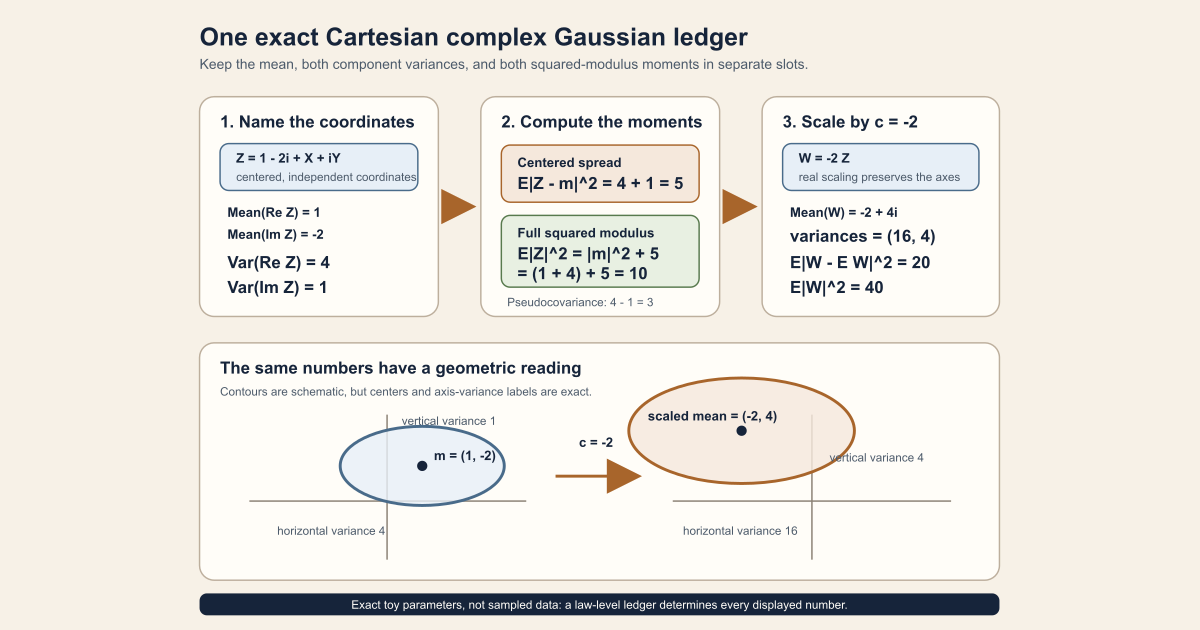
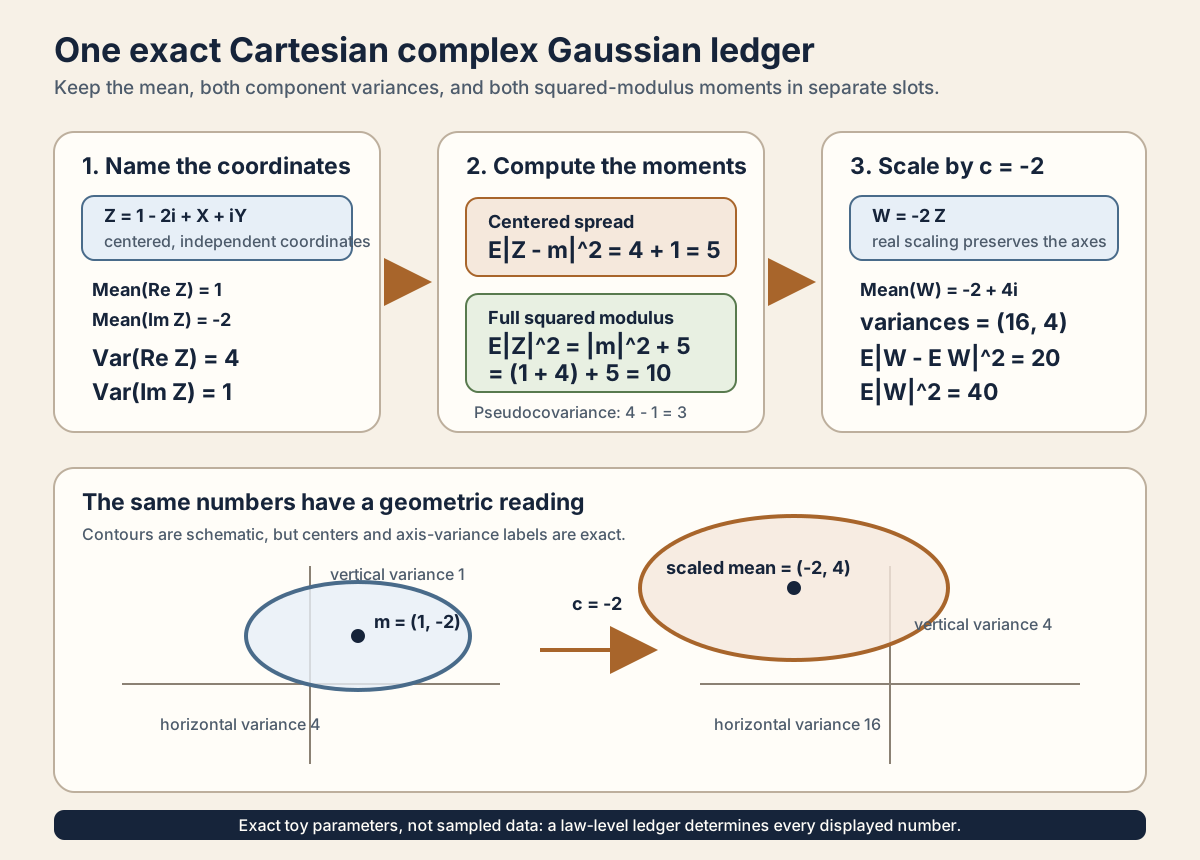
\[ Z=1-2i+X+iY, \]where the two real-valued variables \(X\) and \(Y\) satisfy the following four conditions:
\[ \mathbb E[X]=0, \qquad \mathbb E[Y]=0, \qquad \operatorname{Var}(X)=4, \qquad \operatorname{Var}(Y)=1. \]Assume in addition that \(X\) and \(Y\) are independent and each has an exact real Gaussian law. Then the real and imaginary coordinates of \(Z\) are
\[ \operatorname{Re}Z=1+X, \qquad \operatorname{Im}Z=-2+Y. \]The word mean names the probability-weighted center. The word variance names expected squared displacement from that center. Translation changes a mean but does not change variance, so the first four entries of the ledger are
| Slot | Exact value | Why |
|---|---|---|
| real-coordinate mean | \(1\) | \(1+\mathbb E[X]=1\) |
| imaginary-coordinate mean | \(-2\) | \(-2+\mathbb E[Y]=-2\) |
| real-coordinate variance | \(4\) | adding 1 does not change spread |
| imaginary-coordinate variance | \(1\) | adding \(-2\) does not change spread |
The complex mean is therefore
\[ m=\mathbb E[Z]=1-2i. \]This example is anisotropic: its spread depends on direction because the real-axis variance \(4\) differs from the imaginary-axis variance \(1\). Nothing has been sampled. These are parameters of the whole probability law, not measurements from a scatter plot.
Compute the centered squared-modulus moment
For a complex number \(a+ib\), its squared modulus is \(|a+ib|^2=a^2+b^2\). Since \(Z-m=X+iY\),
\[ \begin{aligned} \mathbb E|Z-m|^2 &=\mathbb E(X^2+Y^2)\\ &=\operatorname{Var}(X)+\operatorname{Var}(Y)\\ &=4+1\\ &=5. \end{aligned} \]The centered squared-modulus moment is the sum of the two component variances. It is not either component variance by itself.
Compute the full squared-modulus moment
The mean contributes its own squared magnitude:
\[ |m|^2=|1-2i|^2=1^2+(-2)^2=5. \]The centered cross terms have expectation zero, so
\[ \begin{aligned} \mathbb E|Z|^2 &=|m|^2+\mathbb E|Z-m|^2\\ &=5+5\\ &=10. \end{aligned} \]This distinction will matter repeatedly: \(5\) measures spread around the mean, while \(10\) measures squared distance from the origin.
Scale the same law by a real number
Set \(W=-2Z\). Real scaling multiplies both coordinate means by \(-2\) and both component variances by \((-2)^2=4\):
\[ \mathbb E[W]=-2+4i, \qquad \bigl(\operatorname{Var}(\operatorname{Re}W), \operatorname{Var}(\operatorname{Im}W)\bigr)=(16,4). \]Consequently,
\[ \mathbb E|W-\mathbb E W|^2=16+4=20, \qquad \mathbb E|W|^2=4\,\mathbb E|Z|^2=40. \]The sign changes the center but the variance scale sees only the square. The exact project scaling theorem later in this chapter includes negative and zero real scalars.
In Lean: name the exact law before asking for moments
HasCartesianComplexGaussianLaw Z (1 - 2 * Complex.I) (4 : ℝ≥0) (1 : ℝ≥0) PHasCartesianComplexGaussianLawis a proposition, so a term of this type is evidence for an exact law rather than a generated sample.Z : Ω → ℂis the sample map from outcomes to complex values.1 - 2 * Complex.Iis the complex mean parameter \(1-2i\).(4 : ℝ≥0)and(1 : ℝ≥0)are separate nonnegative real-coordinate and imaginary-coordinate variances. The type annotation prevents either number from being mistaken for a natural or real scalar in isolation.Pis the source measure. The exact law proposition entails that it is a probability measure; it is not an unnamed default distribution.
The proposition identifies the complete pushforward law. It is stronger than the four moment equalities above. Conversely, the arithmetic equalities alone would not identify a Gaussian law or prove independence.
A nearby nonexample: the same marginals can lie on one line
Let \(U\) be a centered real Gaussian with variance one and form
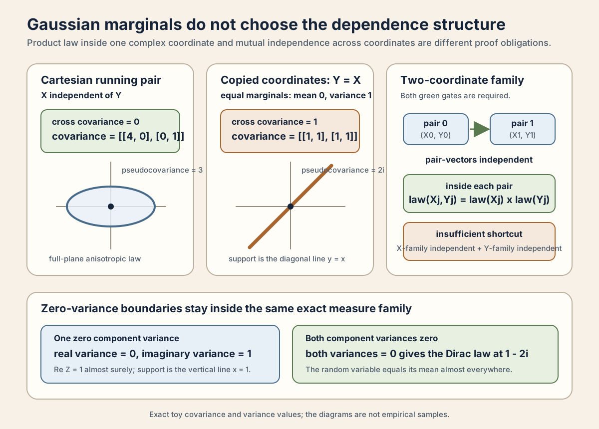
\[ Z_{\mathrm{copy}}=U+iU. \]Both displayed coordinates have the same \(N(0,1)\) marginal law, but they are not independent: learning the real coordinate determines the imaginary one. Here \(N(0,1)\) means the real Gaussian law with mean zero and variance one. The real covariance matrix is
\[ \begin{bmatrix} 1&1\\ 1&1 \end{bmatrix}, \]not the identity matrix. Every realization lies on the diagonal line \(y=x\). Its pseudocovariance, the centered moment \(\mathbb E[Z_{\mathrm{copy}}^2]\), equals
\[ \mathbb E[(U+iU)^2]=2i\,\mathbb E[U^2]=2i. \]Thus equal Gaussian marginals do not certify a Cartesian product law, circular symmetry, or even two-dimensional support. The missing datum is the joint dependence structure.
The dependence question grows when there are several complex coordinates. For \(Z_j=X_j+iY_j\), product structure inside each pair \((X_j,Y_j)\) is one gate. Mutual independence between the pair-vectors is another. Knowing only that the \(X\)-family is independent and the \(Y\)-family is independent leaves every cross-family dependence unspecified.
Type the finite ledger yourself with Lean and Std
The exact Gaussian measure lives in Mathlib, so its proof is a Full project
check that may require substantial disk space and memory. The arithmetic
ledger is a standalone tutorial. The following file imports only Lean’s
Std library and uses integers and natural numbers to check every
displayed finite value, including the copied-coordinate near-miss. Save it as
/tmp/ComplexGaussianLedger.lean on a normal macOS or Linux
computer:
import Std

namespace ComplexGaussianLedger

structure Ledger where
  meanRe : Int
  meanIm : Int
  varRe : Nat
  varIm : Nat
deriving Repr, DecidableEq

def running : Ledger :=
  { meanRe := 1, meanIm := -2, varRe := 4, varIm := 1 }

def centeredSqMoment (ledger : Ledger) : Nat :=
  ledger.varRe + ledger.varIm

def meanNormSq (ledger : Ledger) : Nat :=
  ledger.meanRe.natAbs ^ 2 + ledger.meanIm.natAbs ^ 2

def fullSqMoment (ledger : Ledger) : Nat :=
  meanNormSq ledger + centeredSqMoment ledger

def pseudocovariance
    (varRe varIm : Nat) (crossCovariance : Int) : Int × Int :=
  (Int.ofNat varRe - Int.ofNat varIm, 2 * crossCovariance)

def scale (c : Int) (ledger : Ledger) : Ledger :=
  { meanRe := c * ledger.meanRe
    meanIm := c * ledger.meanIm
    varRe := c.natAbs ^ 2 * ledger.varRe
    varIm := c.natAbs ^ 2 * ledger.varIm }

def scaled : Ledger := scale (-2) running

def copiedCovariance : List (List Nat) :=
  [[1, 1], [1, 1]]

#eval [running.meanRe, running.meanIm]
#eval [running.varRe, running.varIm,
  centeredSqMoment running, fullSqMoment running]
#eval pseudocovariance running.varRe running.varIm 0
#eval [scaled.meanRe, scaled.meanIm]
#eval [scaled.varRe, scaled.varIm,
  centeredSqMoment scaled, fullSqMoment scaled]
#eval pseudocovariance scaled.varRe scaled.varIm 0
#eval copiedCovariance
#eval pseudocovariance 1 1 1

example : centeredSqMoment running = 5 := by decide
example : fullSqMoment running = 10 := by decide
example : pseudocovariance running.varRe running.varIm 0 = (3, 0) := by decide
example : scaled =
    { meanRe := -2, meanIm := 4, varRe := 16, varIm := 4 } := by decide
example : centeredSqMoment scaled = 20 := by decide
example : fullSqMoment scaled = 40 := by decide
example : pseudocovariance 1 1 1 = (0, 2) := by decide

end ComplexGaussianLedger
Type these commands exactly:
source "$HOME/.elan/env"
elan run leanprover/lean4:v4.32.0 lean /tmp/ComplexGaussianLedger.lean
This exact worksheet was executed successfully with Lean 4.32.0. It printed:
[1, -2]
[4, 1, 5, 10]
(3, 0)
[-2, 4]
[16, 4, 20, 40]
(12, 0)
[[1, 1], [1, 1]]
(0, 2)
The first two lines are the running mean pair and its variance, centered-
moment, and full-moment ledger. The next line is its pseudocovariance. The
following three lines repeat those calculations after scaling by \(-2\). The
last two lines are the copied-coordinate covariance matrix and
pseudocovariance. An ordered pair (a, b) represents the complex
number \(a+ib\), so (3, 0) is the running law’s real
pseudocovariance \(3\), while (0, 2) is the copied near-miss’s
\(2i\).
This worksheet checks finite arithmetic and data transformations. It does not define a probability measure, prove Gaussianity or independence, or replace the Mathlib-backed project theorems. Those exact interfaces are identified with full project commands later in the chapter.
A real Gaussian law has one axis. A complex Gaussian law has two. That extra axis creates choices that informal notation often erases: whether the real and imaginary parts are independent, whether their variances agree, whether a quoted variance is per coordinate or total, whether the law has a planar density, and whether rotation invariance is actually known.
This chapter builds one deliberately explicit family. It starts from exact real Gaussian measures, forms their product, and transports the result through the canonical identification of an ordered pair \((x,y)\) with the complex number \(x+iy\). The two component variances remain visible at every stage. That choice covers circular, elliptical, line-supported, and point-mass branches while keeping their distinct geometries explicit.
The Lean module follows the same dependency order. It proves the exact measure first, then coordinate laws and independence, then qualitative Gaussianity and analytic consequences. It does not formalize a density, properness, circularity, the squared-modulus formulas above, or a matrix ensemble. Those boundaries are stated here instead of being hidden behind a suggestive name.
Choose a route up
| Route | Start with | What you will gain |
|---|---|---|
| First encounter | The exact anisotropic ledger | Means, component variances, squared-modulus moments, and scaling from one example |
| Hands-on Lean route | The finite Std worksheet | Run every opening arithmetic check without Mathlib or Lake |
| Probability route | Product laws and pushforwards | Why exact marginals plus independence determine this law |
| Geometry route | Variance along each axis | A complete map of circular, elliptical, line, and point branches |
| Signal route | Covariance and pseudocovariance | A careful separation of properness from circular symmetry |
| Project Lean route | HasLaw and a real-linear equivalence | Human, paper, and exact project syntax with full project commands |
| Random-matrix route | Normalization ledgers | A safe handoff toward complex matrix entries without naming GUE early |
Learning objectives
By the summit, you should be able to:
- reproduce the running ledger’s means, component variances, centered moment \(5\), full squared-modulus moment \(10\), and scaled values;
- define the Cartesian complex Gaussian measure as a pushforward of a product of two exact real Gaussian laws;
- recover its real, imaginary, and joint coordinate laws;
- explain why Gaussian marginals do not encode within-pair or family independence;
- derive the positive-variance planar density without using it at singular variance values;
- compute total centered squared magnitude and pseudocovariance from the two component variances;
- distinguish a proper law from a circularly symmetric law;
- convert between the two common symmetric normalizations;
- explain why
HasLawgives almost-everywhere measurability rather than ordinary measurability; and - identify exactly what the current Lean modules prove and what remains mathematical context.
Base camp: the complex plane is a real two-dimensional space
Every complex number has a unique decomposition
\[ z=x+iy, \qquad x,y\in\mathbb R. \]The maps \(z\mapsto(\operatorname{Re}z,\operatorname{Im}z)\) and \((x,y)\mapsto x+iy\) are inverse real-linear maps. They are also continuous and measurable. This matters because a probability law can be transported in either direction without changing its information, only its representation.
A complex random variable is a map
\[ Z:\Omega\longrightarrow\mathbb C \]on a measured outcome space. Its coordinate pair is
\[ \omega\longmapsto \bigl(\operatorname{Re}Z(\omega),\operatorname{Im}Z(\omega)\bigr). \]Three objects must remain distinct:
| Object | Example | What it records |
|---|---|---|
| Sample map | \(Z:\Omega\to\mathbb C\) | which complex value each outcome produces |
| Realization | \(Z(\omega)\) | one value at one outcome |
| Law | \(\mathcal L_{\mathbb P}(Z)\) | the probability assigned to every measurable region of the plane |
A scatter plot is a finite collection of realizations. It can suggest shape, but it is not the law and does not prove independence, Gaussianity, or rotational symmetry.
Camp one: assemble the exact Cartesian law
Write \(\gamma_{a,v}\) for the real Gaussian law with mean \(a\in\mathbb R\) and variance \(v\ge0\). For a complex center
\[ m=m_{\mathrm R}+i m_{\mathrm I} \]and coordinate variances \(v_{\mathrm R},v_{\mathrm I}\ge0\), begin on \(\mathbb R\times\mathbb R\) with the product measure
\[ \gamma_{m_{\mathrm R},v_{\mathrm R}} \otimes \gamma_{m_{\mathrm I},v_{\mathrm I}}. \]The first factor governs the real coordinate. The second governs the imaginary coordinate. The product sign is the dependence statement: the coordinates are independent. Now transport the pair through
\[ \Phi(x,y)=x+iy. \]The resulting measure is
\[ \Gamma^{\mathrm{cart}}_{m;v_{\mathrm R},v_{\mathrm I}} =\Phi_* \left( \gamma_{m_{\mathrm R},v_{\mathrm R}} \otimes \gamma_{m_{\mathrm I},v_{\mathrm I}} \right). \]In Lean: construct the measure from the product law
((gaussianReal m.re vRe).prod (gaussianReal m.im vIm)).map Complex.equivRealProdCLM.symmgaussianReal m.re vReis the exact real Gaussian measure for the real axis;m.reextracts the real part of the complex mean.gaussianReal m.im vImis the corresponding imaginary-axis measure..prodforms the product measure. This is the measure-level independence choice, not mere side-by-side notation.Complex.equivRealProdCLM.symmis the continuous real-linear map that sends a pair \((x,y)\) to \(x+iy\)..mappushes the product measure through that map. The project definitioncartesianComplexGaussian m vRe vImis exactly this expression.
The dedicated Cartesian complex Gaussian law entry gives the compact operational definition. Here we will unpack every layer.
Why exact marginals are not enough
Suppose \(X\) and \(Y\) are both standard real Gaussian variables. At least two incompatible joint constructions have those marginals:
- choose \(X\) and \(Y\) independently;
- choose one standard Gaussian \(X\) and set \(Y=X\).
In the independent case, \((X,Y)\) fills a two-dimensional cloud. In the copied case, every point lies on the diagonal line \(y=x\). The marginals are identical, but the joint laws, support dimensions, and rotation properties are different.
The Cartesian law chooses the first type of coupling. This is why its definition begins with a product measure rather than merely listing two Gaussian marginals.
The coordinate law can be recovered exactly
Map the complex law back through
\[ z\longmapsto(\operatorname{Re}z,\operatorname{Im}z). \]Because this map is the inverse of \(\Phi\), the original product measure is recovered:
\[ (\operatorname{Re},\operatorname{Im})_* \Gamma^{\mathrm{cart}}_{m;v_{\mathrm R},v_{\mathrm I}} = \gamma_{m_{\mathrm R},v_{\mathrm R}} \otimes \gamma_{m_{\mathrm I},v_{\mathrm I}}. \]Projecting that product onto either coordinate gives the corresponding exact real Gaussian marginal. This back-and-forth identity is stronger than a moment calculation. It identifies the complete probability law.
In Lean: recover the whole coordinate pair, then independence
hZ.indep_re_imhZis evidence ofHasCartesianComplexGaussianLaw Z m vRe vIm P.hZ.jointHasLawreturns an exactHasLawstatement for the pair-valued mapfun ω ↦ ((Z ω).re, (Z ω).im). It does not merely return its two marginals.hZ.indep_re_impackages the resulting within-pair independence as Mathlib’sIndepFunpredicate underP.- The displayed term is exact Lean syntax for the conclusion. The preceding
product-law certificate remains separately available as
hZ.jointHasLaw; both declarations are included in the full project worksheet below.
Camp two: the variance split determines support geometry
The two nonnegative variances form a complete branch table for this family.
Both variances positive: a planar density
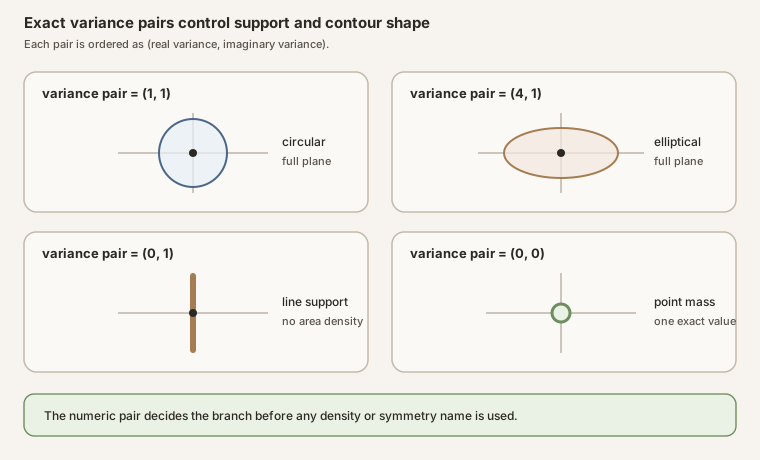
When \(v_{\mathrm R}\gt 0\) and \(v_{\mathrm I}\gt 0\), multiply the two one-dimensional Gaussian densities. The coordinate map \(\Phi\) has unit Jacobian, so with \(z=x+iy\),
\[ f(z) =\frac{1}{2\pi\sqrt{v_{\mathrm R}v_{\mathrm I}}} \exp\!\left( -\frac{(x-m_{\mathrm R})^2}{2v_{\mathrm R}} -\frac{(y-m_{\mathrm I})^2}{2v_{\mathrm I}} \right). \]A level set of the exponent satisfies
\[ \frac{(x-m_{\mathrm R})^2}{v_{\mathrm R}} +\frac{(y-m_{\mathrm I})^2}{v_{\mathrm I}} =\text{constant}. \]These are ellipses aligned with the real and imaginary axes. The larger component variance produces the longer axis.
Equal positive variances: isotropic contours
If \(v_{\mathrm R}=v_{\mathrm I}=q\gt 0\), then
\[ f(z) =\frac{1}{2\pi q} \exp\!\left(-\frac{|z-m|^2}{2q}\right). \]The density depends only on distance from \(m\), so its contours are circles. The centered law is invariant under every rotation. Notice that the total centered squared magnitude will be \(2q\), not \(q\). A component variance and a total complex second moment are different normalization slots.
Exactly one variance zero: a Gaussian line
Suppose \(v_{\mathrm R}=0\) and \(v_{\mathrm I}\gt 0\). The real coordinate equals \(m_{\mathrm R}\) almost surely, while the imaginary coordinate remains Gaussian. The law is supported on the vertical line
\[ \{m_{\mathrm R}+iy:y\in\mathbb R\}. \]The reversed branch gives a horizontal line. Neither law has a density with respect to planar area. It does have a one-dimensional Gaussian description along its supporting line.
Both variances zero: a Dirac mass
When \(v_{\mathrm R}=v_{\mathrm I}=0\), both real coordinate measures are Dirac masses. Their product is a Dirac mass at \((m_{\mathrm R},m_{\mathrm I})\), and the coordinate-pairing map sends that point to \(m\). Therefore
\[ \Gamma^{\mathrm{cart}}_{m;0,0}=\delta_m. \]This is a Gaussian law in Mathlib’s qualitative sense. Degenerate Gaussians are part of the closed family. Excluding them would make scaling by zero an artificial exceptional case.
In Lean: the double-zero branch is exactly Dirac
cartesianComplexGaussian_zero_variances mcartesianComplexGaussian_zero_variances mis the measure-level equality withMeasure.dirac m.hZnow has typeHasCartesianComplexGaussianLaw Z m 0 0 P.hZ.ae_eq_const_of_variances_zerois the sample-map consequence; it uses almost-everywhere equality because exact laws are insensitive to a null-set modification.0 0fills the real and imaginary variance slots separately. No singular density expression or division by a variance appears.
Camp three: mean, total spread, and pseudocovariance
Let
\[ Z=m+X+iY, \]where \(X\sim\gamma_{0,v_{\mathrm R}}\), \(Y\sim\gamma_{0,v_{\mathrm I}}\), and \(X,Y\) are independent. Linearity of integration gives
\[ \mathbb E[Z] =m+\mathbb E[X]+i\mathbb E[Y] =m. \]In Lean: integrability licenses the complex mean
hZ.mean_eqhZ.integrableis the checked analytic gate. A raw integral term alone would not prove that its integrand has finite expected norm.hZ.mean_eqis the exact integral identity∫ ω, Z ω ∂P = m.- The proof uses
Complex.extto reduce equality of complex numbers to equality of their real and imaginary components, then invokes the exact real-coordinate mean theorems. - The displayed term is exact Lean syntax. The separate gate
hZ.integrablealso appears in the full project worksheet later in the page.
Complex second-order theory then splits into two quantities.
Covariance with conjugation measures total squared magnitude
The conventional scalar complex covariance is
\[ C_Z =\mathbb E\!\left[(Z-m)\overline{(Z-m)}\right] =\mathbb E|Z-m|^2. \]Since \(|X+iY|^2=X^2+Y^2\),
\[ C_Z=v_{\mathrm R}+v_{\mathrm I}. \]This nonnegative real number measures total squared spread across both axes.
Pseudocovariance detects directional imbalance
The pseudocovariance is
\[ P_Z =\mathbb E[(Z-m)^2]. \]Expand the square:
\[ (X+iY)^2=X^2-Y^2+2iXY. \]Independence and centering give \(\mathbb E[XY]=\mathbb E[X]\mathbb E[Y]=0\), so
\[ P_Z=v_{\mathrm R}-v_{\mathrm I}. \]The pair \((C_Z,P_Z)\) recovers the two coordinate variances in this Cartesian family:
\[ v_{\mathrm R}=\frac{C_Z+P_Z}{2}, \qquad v_{\mathrm I}=\frac{C_Z-P_Z}{2}. \]Here \(P_Z\) is real because the Cartesian axes are independent. For a general complex Gaussian pair with nonzero covariance between the real and imaginary coordinates, \(P_Z\) can be complex. This is one reason a single scalar called “complex variance” cannot describe every second-order law.
The variance entry explains Mathlib’s real variance totalization and the moment hypotheses that keep zero-variance reasoning explicit.
The properness ridge: a moment condition is not a symmetry definition
A finite-second-moment complex variable is proper when its centered pseudocovariance is zero:
\[ P_Z=0. \]For the Cartesian family,
\[ P_Z=0 \quad\Longleftrightarrow\quad v_{\mathrm R}=v_{\mathrm I}. \]This is a second-order statement. It examines one complex moment.
A centered complex law is circularly symmetric when
\[ e^{i\theta}(Z-m)\stackrel{d}{=}Z-m \qquad\text{for every }\theta\in\mathbb R. \]This is a full-law statement. It asks whether every measurable event keeps the same probability after every rotation.
What implication is safe
If a centered finite-second-moment law is circularly symmetric, then it is proper. Rotating by a phase multiplies the pseudocovariance by \(e^{2i\theta}\); invariance for every angle forces that number to vanish.
The converse fails for arbitrary distributions. A zero pseudocovariance does not fix higher moments or the full angular distribution. One can arrange non-circular discrete laws whose second moment happens to cancel.
Within a centered Gaussian family, the implication is stronger. A Gaussian law is determined by its first and second-order real data. Properness removes the directional second-order imbalance, and the resulting centered law is circularly symmetric. In the Cartesian scalar case, the density above makes the implication visible: equal component variances reduce the exponent to a function of \(|z-m|\) alone.
Centered circularity is not origin circularity
If \(m\ne0\), the centered variable \(Z-m\) may be circularly symmetric, but the law of \(Z\) is generally not invariant under multiplication by a phase about the origin. The rotation moves the mean. A careful statement says either “circularly symmetric about zero” or “the centered law is circularly symmetric.”
What the project name claims
The Lean measure is called cartesianComplexGaussian, not
circularComplexGaussian or
properComplexGaussian. Unequal component variances are allowed,
and no circularity or properness predicate appears in the module. The name
records exactly what is proved: a product in Cartesian coordinates followed by
a real-linear equivalence.
Revisit the running example as a density
The opening parameters were
\[ m=1-2i, \qquad v_{\mathrm R}=4, \qquad v_{\mathrm I}=1. \]The exact coordinate laws are therefore
\[ \operatorname{Re}Z\sim\gamma_{1,4}, \qquad \operatorname{Im}Z\sim\gamma_{-2,1}, \]and their joint law is the product of these two real laws. Because both variances are positive, the planar density exists and equals
\[ f(x+iy) =\frac{1}{4\pi} \exp\!\left( -\frac{(x-1)^2}{8} -\frac{(y+2)^2}{2} \right). \]The coefficient follows from \(1/(2\pi\sqrt{4\cdot1})=1/(4\pi)\). The real standard deviation is \(2\), while the imaginary standard deviation is \(1\), so the contours are twice as wide horizontally at matched standardized radius.
The centered second-order ledger is the one already computed:
\[ C_Z=4+1=5, \qquad P_Z=4-1=3. \]The calculation \(P_Z=3\) shows that this Cartesian Gaussian is not proper and is not circularly symmetric. The checked project law supplies the exact product and marginal data. The density, \(C_Z\), \(P_Z\), properness, and circularity conclusions remain mathematical context rather than named declarations in the current complex-Gaussian module.
The normalization pass: two common circular laws
Let \(U,V\) be independent real standard Gaussians, each with mean zero and variance one.
Unit total squared magnitude
Define
\[ Z_{\mathrm{unit}} =\frac{U+iV}{\sqrt2}. \]Then
\[ v_{\mathrm R}=v_{\mathrm I}=\frac12, \qquad C_Z=1, \qquad P_Z=0, \]and
\[ f_{\mathrm{unit}}(z) =\frac1\pi e^{-|z|^2}. \]Many probability, communications, and random-matrix texts use a notation such as \(\mathcal{CN}(0,1)\) for this total-second-moment convention.
Unit component variances
Define instead
\[ Z_{\mathrm{component}}=U+iV. \]Now
\[ v_{\mathrm R}=v_{\mathrm I}=1, \qquad C_Z=2, \qquad P_Z=0, \]and
\[ f_{\mathrm{component}}(z) =\frac1{2\pi}e^{-|z|^2/2}. \]Both laws are proper and circularly symmetric. They differ by the deterministic factor \(\sqrt2\). A theorem or model that says only “standard complex Gaussian” leaves this factor unresolved.
The normalization convention entry turns this comparison into a reusable ledger. The current formalization keeps \(v_{\mathrm R}\) and \(v_{\mathrm I}\) as separate public parameters and deliberately does not bless either symmetric branch as the matrix-entry convention.
In Lean: real scaling squares both variance factors
hZ.real_smul (-2)hZis again an exact Cartesian-law certificate..real_smulis a theorem inNonlinearDynamics.Random.ComplexGaussianFamilies, even when it is applied to one coordinate. The later module extends the earlier namespace rather than changing the definition of the law.(-2)is a real scalar inferred from the theorem argument.- The conclusion uses the square \((-2)^2\) in both nonnegative variance slots. At scalar zero, the same theorem reaches the double-zero Dirac law.
- The theorem proves an exact law transformation. It does not itself name the squared-modulus moments \(20\) and \(40\); the opening worksheet checks those finite consequences of the variance and mean ledger.
High camp: exact law before qualitative Gaussianity
Mathlib defines a Gaussian measure on a real Banach space by asking that every continuous real-linear functional push it forward to a real Gaussian measure. The complex numbers form a two-dimensional real Banach space, so this definition applies to measures on \(\mathbb C\).
The product of two real Gaussian measures is Gaussian on \(\mathbb R\times\mathbb R\). Mapping that product through the continuous real-linear equivalence \(\Phi\) preserves qualitative Gaussianity. Therefore \(\Gamma^{\mathrm{cart}}_{m;v_{\mathrm R},v_{\mathrm I}}\) is Gaussian in Mathlib’s sense for every nonnegative variance pair, including the degenerate branches.
That qualitative property is valuable, but it forgets the explicit Cartesian parameters. The project therefore keeps this order:
\[ \text{exact Cartesian law with two variances} \quad\Longrightarrow\quad \text{qualitative Gaussian law on }\mathbb C. \]It does not use the qualitative predicate to guess a decomposition or a normalization.
The Lean construction, one layer at a time
The module
NonlinearDynamics.Random.ComplexGaussian begins with the exact
measure:
noncomputable def cartesianComplexGaussian
    (m : ℂ) (vRe vIm : ℝ≥0) : Measure ℂ :=
  ((gaussianReal m.re vRe).prod (gaussianReal m.im vIm)).map
    Complex.equivRealProdCLM.symm
The type \(\mathbb R_{\ge0}\), written ℝ≥0, prevents negative
variances. The map is the inverse of the real-coordinate equivalence, so it
sends \((x,y)\) to \(x+iy\).
Measure-level declarations
| Declaration | Checked statement |
|---|---|
cartesianComplexGaussian | defines the pushforward of the product of exact real Gaussian measures |
instIsProbabilityMeasureCartesianComplexGaussian | the resulting measure has total mass one |
instIsGaussianCartesianComplexGaussian | the measure is Gaussian on the real Banach space underlying \(\mathbb C\) |
cartesianComplexGaussian_map_equivRealProd | mapping back to ordered real coordinates recovers the defining product measure |
cartesianComplexGaussian_map_re | the real marginal is exactly \(\gamma_{m_{\mathrm R},v_{\mathrm R}}\) |
cartesianComplexGaussian_map_im | the imaginary marginal is exactly \(\gamma_{m_{\mathrm I},v_{\mathrm I}}\) |
cartesianComplexGaussian_zero_variances | the double-zero branch is exactly \(\delta_m\) |
The map-back theorem is the structural center. The two marginal theorems are its coordinate shadows. The zero-variance theorem works measure-first, so it never invokes a singular density formula.
The exact random-variable predicate
The project then defines
def HasCartesianComplexGaussianLaw
    (Z : Ω → ℂ) (m : ℂ) (vRe vIm : ℝ≥0)
    (P : Measure Ω) : Prop :=
  HasLaw Z (cartesianComplexGaussian m vRe vIm) P
Mathlib’s HasLaw contains two fields:
AEMeasurable Z P, meaning that \(Z\) agrees almost everywhere with a measurable map; and- the exact pushforward identity
Measure.map Z P = cartesianComplexGaussian m vRe vIm.
It does not provide ordinary Measurable Z. Changing a function on
a null set leaves its law unchanged, so this law-level interface intentionally
lives at the almost-everywhere layer.
Consequences of the exact predicate
| Declaration | Checked statement |
|---|---|
HasCartesianComplexGaussianLaw | packages the exact HasLaw statement |
HasCartesianComplexGaussianLaw.aemeasurable | exposes almost-everywhere measurability |
HasCartesianComplexGaussianLaw.isProbabilityMeasure | the source measure \(P\) is a probability measure |
HasCartesianComplexGaussianLaw.jointHasLaw | the real-imaginary pair has the exact product law |
HasCartesianComplexGaussianLaw.real_hasLaw | the real coordinate has its exact project-level real Gaussian law |
HasCartesianComplexGaussianLaw.imag_hasLaw | the imaginary coordinate has its exact project-level real Gaussian law |
HasCartesianComplexGaussianLaw.indep_re_im | the coordinate functions satisfy IndepFun under \(P\) |
HasCartesianComplexGaussianLaw.hasGaussianLaw | forgets explicit parameters into qualitative Gaussianity |
HasCartesianComplexGaussianLaw.memLp | \(Z\in L^p(P)\) for every extended exponent \(p\ne\infty\), including Mathlib’s \(p=0\) case |
HasCartesianComplexGaussianLaw.integrable | the complex-valued variable is integrable |
HasCartesianComplexGaussianLaw.mean_eq | the Bochner integral of \(Z\) equals \(m\) |
HasCartesianComplexGaussianLaw.ae_eq_const_of_variances_zero | at two zero variances, \(Z=m\) almost everywhere |
HasCartesianComplexGaussianLaw.of_indep_re_im | independent exact real Gaussian coordinates assemble the exact complex law |
These seven measure-level declarations plus the predicate and its twelve namespace declarations are the module’s twenty public declarations.
Independence without invented measurability assumptions
The constructor has the exact shape
theorem HasCartesianComplexGaussianLaw.of_indep_re_im
    {X Y : Ω → ℝ}
    (hX : HasRealGaussianLaw X m.re vRe P)
    (hY : HasRealGaussianLaw Y m.im vIm P)
    (hXY : IndepFun X Y P) :
    HasCartesianComplexGaussianLaw
      (fun ω ↦ X ω + Y ω * Complex.I) m vRe vIm P
There are no separate assumptions Measurable X or
Measurable Y. Each exact real HasLaw supplies the
almost-everywhere measurability needed by the law-composition theorems.
This is compatible with Mathlib’s definition of IndepFun.
Independence of functions is independence of the two measurable spaces pulled
back along those functions using MeasurableSpace.comap. The
property does not itself assert that either function is measurable from the
ambient measurable space on \(\Omega\). When almost-everywhere measurability is
needed to identify the joint pushforward law, the two exact law hypotheses
supply it.
The proof proceeds in two conceptual steps:
hXY.hasLaw_prod hX hYproves that \(\omega\mapsto(X(\omega),Y(\omega))\) has the product law;- composition with
Complex.equivRealProdCLM.symmturns the pair into \(X+iY\) and maps the product tocartesianComplexGaussian.
This is the proof-level version of the glossary figure: establish the joint coordinate law, then change representation.
Analytic consequences and their exact boundary
The module obtains finite \(L^p\) membership and integrability from
qualitative HasGaussianLaw. The statement
MemLp Z p P for every p != infinity
includes every positive finite moment order and Mathlib’s special \(p=0\) case. It does not claim essential boundedness, which would correspond to \(p=\infty\). Positive-variance Gaussian laws have unbounded support.
The mean theorem proves a complex Bochner integral identity by applying
Complex.ext and reducing to the already checked real and imaginary
mean theorems. Integrability justifies moving each coordinate through the
integral.
The module stops before a named complex variance. That is intentional.
Mathlib’s real variance API and the signal-processing quantities
\(C_Z\) and \(P_Z\) have different types and conventions. A future formal
layer must define the desired complex second moments explicitly, prove their
integrability, and then establish the sum and difference formulas.
Full project check of the exact single-coordinate interfaces
The authoritative source is
formalization/NonlinearDynamics/Random/ComplexGaussian.lean.
After installing the repository’s pinned dependencies, put these lines in a
temporary project scratch file:
import NonlinearDynamics.Random.ComplexGaussian

open MeasureTheory ProbabilityTheory
open scoped ENNReal NNReal ProbabilityTheory
open NonlinearDynamics.Random

#print cartesianComplexGaussian
#check instIsProbabilityMeasureCartesianComplexGaussian
#check instIsGaussianCartesianComplexGaussian
#check cartesianComplexGaussian_map_equivRealProd
#check cartesianComplexGaussian_map_re
#check cartesianComplexGaussian_map_im
#check cartesianComplexGaussian_zero_variances
#print HasCartesianComplexGaussianLaw
#check HasCartesianComplexGaussianLaw.aemeasurable
#check HasCartesianComplexGaussianLaw.isProbabilityMeasure
#check HasCartesianComplexGaussianLaw.jointHasLaw
#check HasCartesianComplexGaussianLaw.real_hasLaw
#check HasCartesianComplexGaussianLaw.imag_hasLaw
#check HasCartesianComplexGaussianLaw.indep_re_im
#check HasCartesianComplexGaussianLaw.hasGaussianLaw
#check HasCartesianComplexGaussianLaw.memLp
#check HasCartesianComplexGaussianLaw.integrable
#check HasCartesianComplexGaussianLaw.mean_eq
#check HasCartesianComplexGaussianLaw.ae_eq_const_of_variances_zero
#check HasCartesianComplexGaussianLaw.of_indep_re_im
#print exposes a definition body. #check
elaborates an existing declaration and displays its type. Neither command draws
samples, estimates a moment, proves circular symmetry, or upgrades the
unformalized density and pseudocovariance formulas. The full project command below
checks the authoritative module under Lean 4.32.0 and pinned Mathlib 4.32.0.
cd formalization
lake env lean -DwarningAsError=true NonlinearDynamics/Random/ComplexGaussian.lean
Resource note: this exact file uses the repository's
pinned Lean and Mathlib dependencies. Initial project setup can require
substantial disk space and build time. For a lightweight first step on
macOS or Linux, use the page's standalone Lean-core or Std
tutorial.
Full project check of the scaling and family interfaces
The authoritative continuation is
formalization/NonlinearDynamics/Random/ComplexGaussianFamilies.lean.
The next temporary project scratch file checks the exact scaling and
independence-scope names used in this chapter:
import NonlinearDynamics.Random.ComplexGaussianFamilies

open MeasureTheory ProbabilityTheory
open scoped ENNReal NNReal ProbabilityTheory
open NonlinearDynamics.Random

#check HasCartesianComplexGaussianLaw.real_smul
#print IndependentCartesianComplexGaussianFamily
#check IndependentCartesianComplexGaussianFamily.measurable
#check IndependentCartesianComplexGaussianFamily.hasLaw
#check IndependentCartesianComplexGaussianFamily.independent
#check IndependentCartesianComplexGaussianFamily.real_variance_eq
#check IndependentCartesianComplexGaussianFamily.imag_variance_eq
#check IndependentCartesianComplexGaussianFamily.of_independent_real_pair_laws
#check IndependentCartesianComplexGaussianFamily.scale
The first declaration is the exact single-coordinate real-scaling theorem. The structure print shows that coordinate measurability, each coordinate’s exact Cartesian law, and mutual family independence occupy separate fields. The constructor from real pair-vectors requires an exact product law inside every pair and independence between pair-vectors. It never infers cross-family independence from two separately independent real families. This exact file imports Mathlib and the project, so checking it may require substantial disk space and memory.
cd formalization
lake env lean -DwarningAsError=true NonlinearDynamics/Random/ComplexGaussianFamilies.lean
Resource note: this exact file uses the repository's
pinned Lean and Mathlib dependencies. Initial project setup can require
substantial disk space and build time. For a lightweight first step on
macOS or Linux, use the page's standalone Lean-core or Std
tutorial.
The deliberate RMT-03 boundary before a family
The single-coordinate layer provides:
- an exact complex probability measure with explicit component variances;
- exact real, imaginary, and joint coordinate laws;
- independence of the two Cartesian coordinates;
- a constructor from independent exact real Gaussian variables;
- qualitative Gaussianity on \(\mathbb C\);
- finite moments, integrability, and exact mean;
- a checked double-zero point-mass theorem, while the one-zero line geometry remains an explicit mathematical consequence of the exact product measure; and
- no hidden selection between the two common circular scales.
It does not itself provide:
- a preferred symmetric variance pair;
- a formal pseudocovariance or properness predicate;
- a proof of circular symmetry;
- a complex density theorem;
- a family of mutually independent complex coordinates;
- a Hermitian matrix constructor;
- a Gaussian unitary ensemble law;
- unitary invariance;
- eigenvalue measurability;
- expected trace moments; or
- an asymptotic spectral theorem.
In Lean: family independence is a separate field
IndependentCartesianComplexGaussianFamily Z m vRe vIm PZ : ι → Ω → ℂis an indexed family of sample maps.m,vRe, andvImare indexed parameter ledgers, so every coordinate retains its own mean and two variances.- The structure field
measurablestores ordinary measurability of every complex coordinate. This is stronger than the almost-everywhere measurability in each exact law. - The field
hasLawstores the single-coordinate Cartesian product law, including within-pair real-imaginary independence. - The field
independentstores Mathlib’siIndepFun Z Pfor the complex coordinates as a family. It is not inferred from the two real component families separately.
A complex matrix law adds diagonal and off-diagonal roles, conjugate reflection, dimension scaling, and a zero-size policy. In a Hermitian matrix, the lower-triangular entries are not independent primitive degrees of freedom: conjugate symmetry determines them from the upper triangle. A later constructor must select primitive coordinates first and reflect them second.
The normalization ledger must then state, at minimum:
| Slot | Required decision |
|---|---|
| Matrix size | index type, dimension, and the zero-dimensional policy |
| Diagonal coordinates | exact real mean and variance |
| Off-diagonal coordinates | exact real-part and imaginary-part means and variances |
| Independence | exactly which primitive upper-triangular coordinates are mutually independent |
| Hermitian reflection | how lower-triangular entries are determined |
| Matrix scaling | every dimension-dependent factor |
| Trace convention | raw trace or normalized trace |
| Spectral target | intended eigenvalue scale |
The word “Gaussian” fills none of these matrix slots by itself.
Common wrong turns
| Wrong turn | Why it fails | Correct layer |
|---|---|---|
| “Both coordinates are Gaussian, so they are independent” | marginals do not determine a coupling | state or prove the joint product law |
| “Complex variance is a single scalar with no convention attached” | component variances, total squared magnitude, and pseudocovariance differ | publish a normalization ledger |
| “Equal variances imply circularity” | not for an arbitrary non-Gaussian joint law | require the full Gaussian product structure |
| “Proper means circular by definition” | properness is second-order; circularity is distributional | use the Gaussian implication only with its hypotheses |
| “A nonzero mean circular Gaussian is origin invariant” | rotations move the mean | center first or state symmetry about \(m\) |
| “The density works at zero variance” | singular laws have no planar density | use the measure definition and Dirac branches |
| “HasLaw proves ordinary measurability” | it stores only almost-everywhere measurability | keep the layers distinct |
| “HasGaussianLaw remembers the component variances” | it is qualitative | retain the exact Cartesian predicate |
| “Standard complex Gaussian fixes the scale” | unit total spread and unit component spread differ by \(\sqrt2\) | keep both variances explicit |
| “A complex coordinate already defines GUE” | a matrix ensemble needs many additional choices and proofs | complete the matrix ledger first |
Summit checklist
- The complex law is defined as a measure, not only by a positive-density formula.
- The real and imaginary means and variances are explicit.
- Independence is encoded in the joint law, not inferred from marginals.
- Every zero-variance branch has a support description.
- Total centered squared magnitude and pseudocovariance are not conflated.
- Properness and circular symmetry are defined at their correct levels.
- A nonzero mean is centered before claiming phase invariance.
- Any “unit” or “standard” scale states whether it is per component or total.
- Single-coordinate Lean claims are limited to the twenty declarations in
ComplexGaussian.lean; scaling and family claims are explicitly attributed toComplexGaussianFamilies.lean. - Density, symmetry, matrix, spectral, and asymptotic claims are not attributed to Lean before they are formalized.
Where to continue
Use the linked glossary as a concept map:
- Cartesian complex Gaussian law for the compact exact definition and branch table;
- Independent Cartesian complex Gaussian family for the checked indexed bundle and dependence contract;
- Gaussian distribution for each real coordinate and its zero-variance Dirac branch;
- independence for product-law factorization;
- variance for squared spread and finite-moment hypotheses;
- normalization convention for the scale ledger; and
- probability law and pushforward measure for the underlying measure transport.
The earlier chapter Gaussian Laws, Independence, and Normalization constructs the exact real laws and finite product machinery used here. Finite Product Probability Spaces and Independent Gaussian Fields continues from one complex coordinate to exact finite field laws, canonical sample spaces, scaling, and the cross-family independence audit. Random Matrices: From Outcomes to Spectra explains the measurable matrix, Hermitian, law, and trace-observable layers that a future Gaussian matrix constructor must join.
References
Mathlib contributors.
Complex numbers as a real normed space,
Mathlib 4 documentation. This official API documents
Complex.equivRealProdCLM, its inverse, and the continuous real and
imaginary coordinate maps.
Mathlib contributors. Gaussian distributions over the reals, Mathlib 4 documentation. This is the exact source for the two coordinate measures, their variances, transformations, moments, and Dirac boundary.
Mathlib contributors. Gaussian distributions in Banach spaces, Mathlib 4 documentation. This defines a Gaussian measure through all continuous real-linear functionals and proves preservation under continuous linear maps and products.
Mathlib contributors. Gaussian random variables, Mathlib 4 documentation. This is the official API for qualitative Gaussian laws, finite \(L^p\) membership, integrability, and continuous linear maps.
Mathlib contributors.
Law of a random variable,
Mathlib 4 documentation. This documents the almost-everywhere measurability
and pushforward identity stored by HasLaw.
Mathlib contributors.
Independence of functions,
Mathlib 4 documentation. This documents the comap-based definition of
IndepFun and its product-law characterization.
Nathaniel R. Goodman. Statistical Analysis Based on a Certain Multivariate Complex Gaussian Distribution, The Annals of Mathematical Statistics 34 (1963), 152-177. This primary historical source develops a circular complex multivariate Gaussian family. It does not determine the normalization chosen by this project.
F. D. Neeser and J. L. Massey. Proper Complex Random Processes with Applications to Information Theory, IEEE Transactions on Information Theory 39 (1993), 1293-1302. This primary source separates covariance from pseudocovariance and defines properness by vanishing pseudocovariance.
Bernard Picinbono. Second-Order Complex Random Vectors and Normal Distributions, IEEE Transactions on Signal Processing 44 (1996), 2637-2640. This primary source explains why covariance alone is insufficient for general complex second-order Gaussian structure.
The exact upstream Lean source audited for this chapter is Mathlib commit
81a5d257,
the dependency revision recorded in formalization/lake-manifest.json.