Start with a moving stable orbit
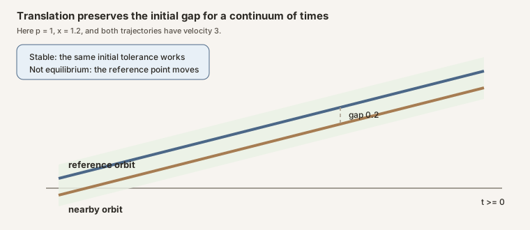
Fix \(c=3\) and define a flow on the real line by
\[ \Phi(t,x)=x+3t. \]Take \(p=1\) and \(x=1.2\). For every real time,
\[ |\Phi(t,x)-\Phi(t,p)|=|(1.2+3t)-(1+3t)|=0.2. \]One initial error stays unchanged for the complete orbit. The reference point is forward stable. It is not an equilibrium, since \(\Phi(1,p)=p+3\ne p\).
The quantifiers define the property
For a flow \(\Phi:\mathbb R\times X\to X\) on a metric space, forward stability at \(p\) means
\[ \forall\varepsilon\gt0\;\exists\delta\gt0\;\forall x, d(x,p)\lt\delta\Longrightarrow \forall t\ge0,\quad d(\Phi(t,p),\Phi(t,x))\lt\varepsilon. \]The same \(\delta\) must control every nonnegative real time. Proving continuity separately for each fixed \(t\) would permit a time-dependent radius and would not establish this statement.
The formal definition uses equicontinuity of the family \((\Phi_t)_{t\ge0}\). A uniform space supplies a notion of closeness without choosing a metric; a pseudo-metric space recovers the displayed formula.
Equilibrium freezes the reference orbit
An equilibrium \(p\) satisfies
\[ \Phi(t,p)=p\qquad\text{for every }t\in\mathbb R. \]For a real flow, it is enough to check nonnegative times. If \(t\lt0\), apply the positive-time identity at \(-t\) and the composition law \(\Phi(t,\Phi(-t,p))=\Phi(0,p)\).
At an equilibrium, forward stability reduces to
\[ d(x,p)\lt\delta\Longrightarrow d(\Phi(t,x),p)\lt\varepsilon \quad(t\ge0). \]The project calls the conjunction IsLyapunovStableEquilibrium.
Attraction asks for approach
An orbit from \(x\) is attracted to \(p\) when
\[ \Phi(t,x)\to p\qquad\text{as }t\to+\infty. \]This is not an all-time error bound. A converging trajectory may have a large transient before it enters and remains in a small neighborhood. The basin of attraction collects the starts with this limit.
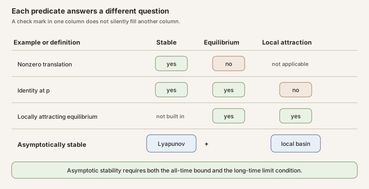
The identity flow supplies a checkable non-example. Every point is a stable equilibrium, but the orbit from \(x\ne p\) is the constant function \(x\), so it does not approach \(p\).
Why an orbit limit is an equilibrium
Suppose \(X\) is Hausdorff and \(\Phi(t,x)\to p\). Fix a time \(s\). Continuity of the map (y\mapsto\Phi(s,y)) gives
\[ \Phi(s,\Phi(t,x))\longrightarrow\Phi(s,p). \]The flow law rewrites the left side as (\Phi(s+t,x)). Translating real time by the fixed amount \(s\) does not change the \(t\to+\infty\) limit, so the same expression also tends to \(p\). Hausdorff uniqueness of limits yields \(\Phi(s,p)=p\). Since \(s\) was arbitrary, \(p\) is an equilibrium.
This argument uses the topological flow structure. It does not infer Lyapunov stability from attraction.
Asymptotic stability combines two obligations
A locally attracting equilibrium has a basin containing a neighborhood of \(p\). An asymptotically stable equilibrium is both Lyapunov stable and locally attracting:
\[ \operatorname{AsympStable}(p) \iff \operatorname{LyapStable}(p) \land B(p)\in\mathcal N(p). \]This interface controls initial perturbations of the state under one fixed flow. It does not compare nearby vector fields or random perturbations.
In Lean
def IsForwardStableAt [UniformSpace X] (ϕ : Flow ℝ X) (p : X) : Prop := EquicontinuousAt (fun t : AddSubmonoid.nonneg ℝ ↦ ϕ t) pAddSubmonoid.nonneg ℝ is the type of pairs consisting of a real number and
a proof that it is nonnegative. EquicontinuousAt chooses one neighborhood
before quantifying over that whole time index.theorem IsAttractedTo.isEquilibrium [TopologicalSpace X] [T2Space X] (hxp : IsAttractedTo ϕ x p) : IsEquilibrium ϕ pT2Space X is the Hausdorff separation assumption used for uniqueness of
limits. Flow.continuous_toFun transports the limit through one time slice,
and Flow.map_add rewrites the transported orbit as a shifted orbit.Try it in the repository
import NonlinearDynamics.Deterministic.ODE.Stability

open NonlinearDynamics.Deterministic.ODE

#check isForwardStableAt_iff_dist
#check isLyapunovStableEquilibrium_iff_dist
#check isEquilibrium_iff_nonneg
#check IsAttractedTo.isEquilibrium
#check isAttractedTo_id_iff
#check forwardStableAt_translationFlow_not_equilibrium
This is a full project check on macOS or Linux. It uses the repository’s pinned Lean and Mathlib dependencies and may require substantial disk space or build time.
cd formalization
lake env lean -DwarningAsError=true NonlinearDynamics/Deterministic/ODE/Stability.lean
Resource note: this exact file uses the repository's
pinned Lean and Mathlib dependencies. Initial project setup can require
substantial disk space and build time. For a lightweight first step on
macOS or Linux, use the page's standalone Lean-core or Std
tutorial.
cd formalization
lake env lean -DwarningAsError=true \
  NonlinearDynamics/Deterministic/ODE/Stability.lean
What this chapter does not claim
No theorem here supplies an attraction rate, exponential stability, an invariant-set stability theory, a Lyapunov function, stable manifolds, structural stability, or robustness to stochastic perturbations. The metric theorems allow pseudo-metrics, so zero distance need not imply equality unless stronger separation assumptions are present.
Related trail markers
- Continuous-time stability
- Forward stability in discrete time
- Basin of attraction
- Stability and Attraction for ODE Flows in Lean
References
- N. P. Bhatia and G. P. Szegő, Dynamical Systems: Stability Theory and Applications, Lecture Notes in Mathematics 35, Springer, 1967. Publisher record.
- J. P. LaSalle, The Stability of Dynamical Systems, SIAM CBMS 25, 1976. Publisher record.
- Mathlib contributors,
Mathlib.Dynamics.Flow, version 4.32.0. - Mathlib contributors,
Topology.UniformSpace.EquicontinuityandTopology.MetricSpace.Equicontinuity, version 4.32.0.