Start with a two-state orbit you can calculate
Let
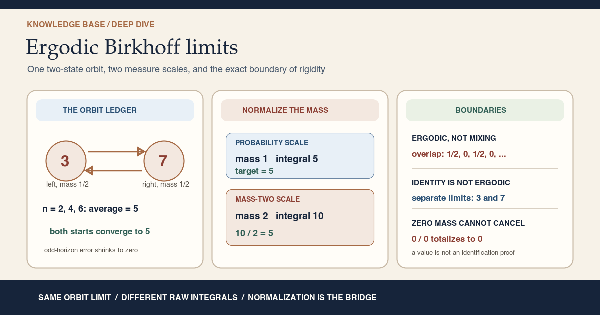
\[ \Omega=\{\mathsf{left},\mathsf{right}\}, \qquad \mu(\{\mathsf{left}\})=\mu(\{\mathsf{right}\})=\frac12. \]The total mass is one, so \(\mu\) is a probability measure . Let the map \(T\) swap the two states, and choose the real observable
\[ f(\mathsf{left})=3, \qquad f(\mathsf{right})=7. \]For a positive horizon \(n\), the Birkhoff average is
\[ A_nf(\omega) {} = \frac1n\sum_{j=0}^{n-1}f\bigl(T^j\omega\bigr). \]The project totalizes the horizon-zero value as \(A_0f=0\). The first seven values, including that bookkeeping term, are
| \(n\) | \(A_nf(\mathsf{left})\) | \(A_nf(\mathsf{right})\) |
|---|---|---|
| 0 | \(0\) | \(0\) |
| 1 | \(3\) | \(7\) |
| 2 | \(5\) | \(5\) |
| 3 | \(13/3\) | \(17/3\) |
| 4 | \(5\) | \(5\) |
| 5 | \(23/5\) | \(27/5\) |
| 6 | \(5\) | \(5\) |
Every positive even horizon contains the same number of threes and sevens, so its average is exactly five. At odd horizon \(2m+1\),
\[ \begin{aligned} A_{2m+1}f(\mathsf{left}) &=5-\frac{2}{2m+1},\\ A_{2m+1}f(\mathsf{right}) &=5+\frac{2}{2m+1}. \end{aligned} \]Both rows therefore converge to five. The probability integral gives the same number:
\[ \int_\Omega f\,d\mu {} = \frac12\cdot3+\frac12\cdot7 {} =5. \]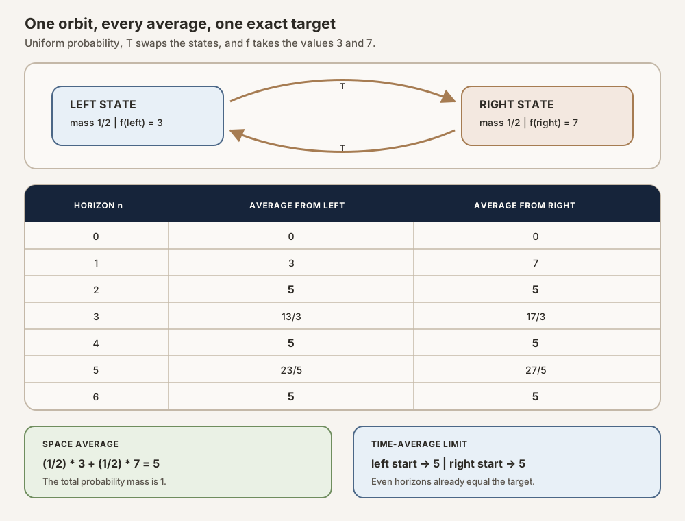
Change only the measure scale
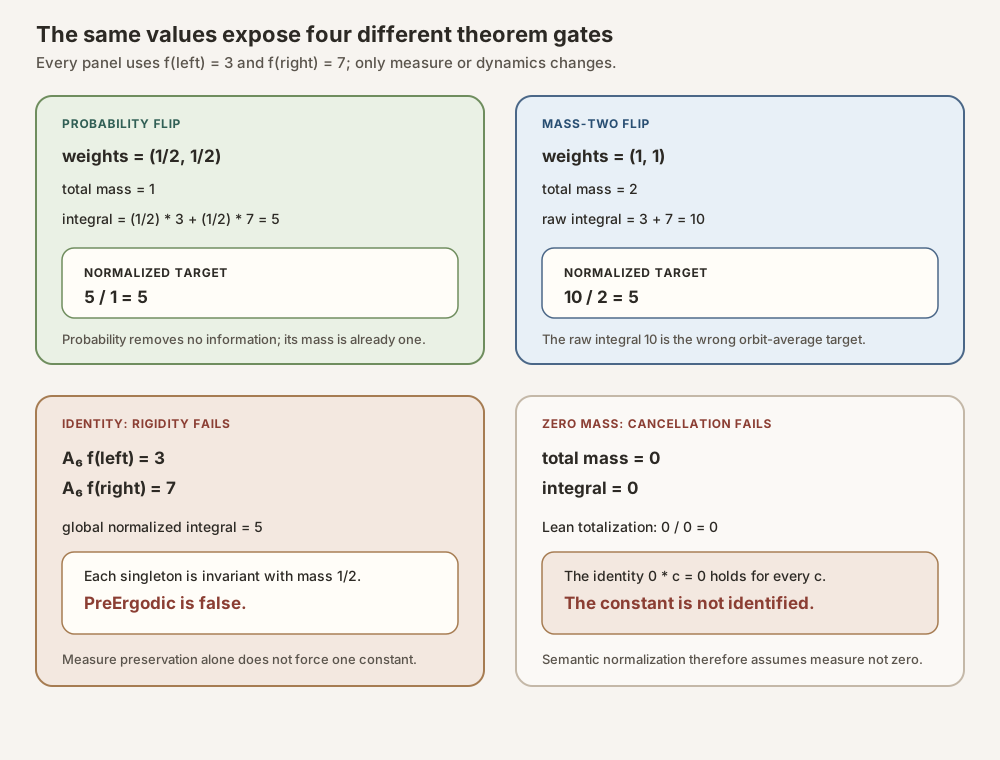
Now give each state mass one instead of one half. The dynamics and orbit averages do not change, but the total mass and raw integral do:
\[ \nu(\Omega)=2, \qquad \int_\Omega f\,d\nu=3+7=10. \]The orbit limit is still five. The correct finite-mass target is therefore
\[ \frac{1}{\nu(\Omega)}\int_\Omega f\,d\nu {} = \frac12\cdot10 {} =5, \]not the raw integral \(10\). Probability normalization is a convenient special case, not a hidden rescaling performed by integration.
Keep three nearby failures visible
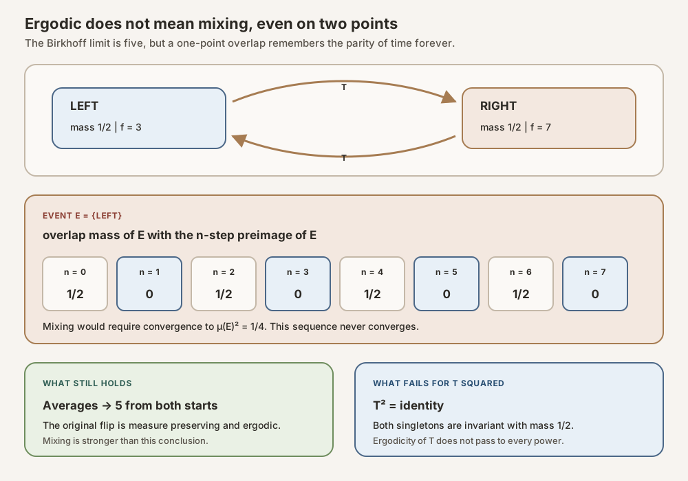
- Ergodic need not mean mixing. For \(E=\{\mathsf{left}\}\), the overlap masses \(\mu(E\cap T^{-n}E)\) for \(n=0,\ldots,7\) are \[ \frac12,0,\frac12,0,\frac12,0,\frac12,0. \] Mixing would require convergence to \(\mu(E)^2=1/4\).
- Preservation need not mean ergodicity. Replace the swap by identity dynamics. Both singleton events are invariant with mass \(1/2\), and the horizon-six averages remain \(3\) and \(7\). They do not collapse to the global mean \(5\).
- Ergodic need not mean positive mass. Under the zero measure, the integral and total mass are both zero. Lean’s total arithmetic evaluates \(0^{-1}\cdot0\) as zero, but the equation \(0\cdot c=0\) identifies no constant. The semantic normalization theorem therefore keeps \(\mu\ne0\) explicit.
From the finite ledger to the theorem
Consider one nonlinear system over a long orbit. Measure one observable at each step. Average those measurements. When should that time average equal the average obtained by sampling the whole state space at once?
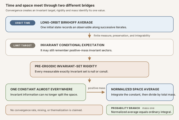
This question links dynamics to statistical physics. A microscopic trajectory moves through phase space, while a macroscopic prediction is often expressed as a space or ensemble average. The bridge has explicit gates: measure preservation supplies stationary orbit sampling, RMT-27 supplies a pointwise limit, pre-ergodic rigidity removes nonconstant invariant information, integrability legitimizes the observable, and finite nonzero mass sets the normalization.
Fix a measurable space \(\Omega\), a finite measure \(\mu\), a self-map \(T:\Omega\to\Omega\), and an integrable real observable \(f:\Omega\to\mathbb R\). RMT-27 proves, under measure preservation, that
\[ A_n f(\omega) \longrightarrow \mu[f\mid\mathcal I_T](\omega) \quad\text{for }\mu\text{-almost every }\omega, \]where \(\mathcal I_T\) is Mathlib’s exact invariant sigma algebra and the right side is conditional expectation . A nonergodic target may still vary between invariant components.
RMT-28 adds the rigidity step. On a finite nonzero measure, if the system is ergodic, then
\[ A_n f(\omega) \longrightarrow \frac{1}{\mu(\Omega)}\int_\Omega f\,d\mu \quad\text{for }\mu\text{-almost every }\omega. \]The right side is the normalized space average . If \(\mu\) is a probability measure, then \(\mu(\Omega)=1\), so the target is the ordinary integral and may be called the expectation of \(f\).
The formalization separates two assumptions. Collapsing an already invariant
conditional expectation to a constant needs only
PreErgodic T μ. Convergence of orbit averages also needs measure
preservation, so the final two Birkhoff theorems use the fuller
Ergodic T μ structure.
The immediate predecessor is Birkhoff Limits, Invariant Sigma Algebras, and Conditional Expectation. The earlier assumption-separation chapter is Probability Normalization and Ergodic Rigidity Before Kingman. The later subadditive consumer is Subadditive Upper Limsup Bounds Before Kingman Convergence, which applies this probability-integral endpoint only under the original map and proves an upper estimate rather than full Kingman convergence. The compact companion is ergodicity .
Choose a route up
| Route | Begin | Destination |
|---|---|---|
| Worked-example route | Start with a two-state orbit you can calculate | Compute every finite average and the exact limit |
| Physical route | Time and space answer different questions | Translate the theorem into dynamics and statistical physics |
| Boundary route | Keep three nearby failures visible | Separate nonmixing, missing rigidity, and zero mass |
| Rigidity route | Pre-ergodic is the exact constancy gate | Separate information collapse from measure preservation |
| Normalization route | The canonical space average | Understand ⨍, finite mass, and probability |
| Proof route | The five proof moves | Derive the constant from conditional expectation |
| Lean route | The exact declaration map | Audit six public declarations, one private proof hinge, and fourteen private boundary fixtures |
| Runnable route | Run the finite worksheet on Mac or Linux | Execute the complete numerical model with only Lean Std |
| Compiled-boundary route | Five compiled boundary probes | Test every weak assumption boundary |
| Practice route | Thirty solved exercises | Rebuild the chapter independently |
Learning objectives
By the summit, a reader should be able to:
- distinguish an orbit time average from a normalized measure-space average;
- state the finite nonzero ergodic Birkhoff target;
- explain why probability is a specialization rather than a hidden premise;
- distinguish
PreErgodicfromErgodic; - explain why conditional-expectation collapse needs only pre-ergodicity;
- explain why orbit convergence still needs measure preservation;
- distinguish an exact invariant sigma algebra from triviality modulo null sets;
- derive the constant by integrating an almost-everywhere equality;
- read Mathlib’s canonical notation
⨍ ω, f ω ∂μ; - compute Birkhoff averages on a two-cycle;
- prove that the cycle is ergodic but not mixing;
- explain why \(T^2\) need not be ergodic when \(T\) is;
- locate where integrability and nonzero mass are consumed;
- audit all six public declarations, the private proof hinge, and fourteen private boundary fixtures;
- explain all five compiled boundary probes;
- run the complete finite
Stdworksheet on a normal Mac or Linux host; and - state every major nonclaim without crossing into Kingman or Oseledets.
Time and space answer different questions
A deterministic orbit begins from one state and produces
\[ \omega,\ T\omega,\ T^2\omega,\ldots. \]The time average \(A_nf(\omega)\) asks what one trajectory records during its first \(n\) observations. The space average asks what the measure assigns across all states:
\[ \text{time: }\frac{1}{n}\sum_{j=0}^{n-1}f(T^j\omega), \qquad \text{space: }\frac{1}{\mu(\Omega)}\int_\Omega f\,d\mu. \]In Hamiltonian mechanics, \(\Omega\) may be an energy surface and \(f\) a macroscopic observable. In a random dynamical system, \(\omega\) may encode an environment shift. In symbolic dynamics, \(f\) may indicate a local pattern. The theorem supplies the same measure-theoretic bridge in each setting. It does not prove that a particular physical system is ergodic, thermalizes quickly, or carries the physically correct equilibrium measure.
Why the nonergodic limit can retain memory
If \(\Omega\) splits into two positive-measure invariant regions, an orbit starting in one cannot sample the other. A long time average may settle to one value on the first region and a different value on the second. The invariant sigma algebra records that surviving information, and conditional expectation onto it is the correct general target.
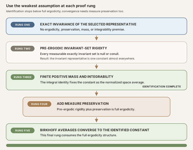
Pre-ergodicity says no measurable strictly invariant region has both it and its complement of positive measure. An invariant measurable real function therefore cannot retain two positive-measure sectors. It is constant almost everywhere.
The result is not a finite-time guarantee
The theorem is asymptotic and almost everywhere. It gives no horizon sufficient for a requested accuracy and permits an exceptional null set of starting states. Slow convergence and long finite-time oscillation are compatible with the theorem.
Pre-ergodic is the exact constancy gate
Mathlib separates two structures. PreErgodic T μ says every
measurable set \(S\) satisfying
is almost empty or almost full. Equivalently, either \(\mu(S)=0\) or \(\mu(S^{\mathsf c})=0\). This is an invariant-information condition. Its definition does not assert that \(T\) preserves \(\mu\).
Ergodic T μ extends both
MeasurePreserving T μ μ; andPreErgodic T μ.
Now set
\[ g=\mu[f\mid\mathcal I_T]. \]This selected conditional-expectation representative is measurable for \(\mathcal I_T\) and satisfies the literal equality
\[ g\circ T=g. \]In Lean: prove exact invariant composition
condExp_invariants_comp (T := T) (f := f) (μ := μ)μ[f | MeasurableSpace.invariants T]is Mathlib’s selected real conditional-expectation representative.∘ Tmeans compose that representative with the base map.(T := T),(f := f), and(μ := μ)supply implicit arguments by name.- The equality sign is literal function equality, not almost-everywhere equality.
- The theorem needs no measure preservation, pre-ergodicity, finiteness, or integrability premise.
Once those facts are available, pre-ergodicity alone makes \(g\) almost everywhere constant. Measure preservation returns only when the RMT-27 orbit-convergence theorem is invoked.
The invariant sigma algebra is not literally bottom
Ergodicity does not generally imply the literal set equation
\[ \mathcal I_T=\{\varnothing,\Omega\}. \]There may be nonempty invariant null sets and proper conull invariant sets.
Pre-ergodicity makes them trivial modulo \(\mu\); it does not delete them as
sets. RMT-28 proves almost-everywhere constancy and never rewrites
MeasurableSpace.invariants T to the bottom measurable space.
Zero measure exposes the boundary
Under the zero measure, every measurable set is both almost empty and almost
full. Mathlib can therefore regard a measurable map as ergodic for zero
measure. RMT-28 keeps hμ : μ ≠ 0 explicit on finite-mass
normalization theorems. Probability measures obtain nonzeroness automatically.
The canonical space average
Mathlib already names the normalized integral:
⨍ ω, f ω ∂μ
On a finite measure,
\[ \operatorname{Avg}_\mu(f) {} = \bigl(\mu.\operatorname{real}(\Omega)\bigr)^{-1} \int_\Omega f\,d\mu. \]In Lean: identify the canonical average
condExp_invariants_ae_eq_average_of_preErgodic hμ hT hfhμ : μ ≠ 0is the nonzero-mass gate.hT : PreErgodic T μsupplies invariant-function rigidity without measure preservation.hf : Integrable f μlicenses the conditional-expectation integral identity that determines the constant.⨍ x, f x ∂μis the Lean notation for Mathlib’s canonical integral average.=ᵐ[μ]means equality outside a \(\mu\)-null set.
The finite nonzero hypotheses make the real denominator legitimate. The proof
first identifies the constant with Mathlib’s canonical average using
measure_smul_average, then exposes the reciprocal-mass form using
average_eq.
In Lean: expose the total-mass normalization
condExp_invariants_ae_eq_normalizedIntegral_of_preErgodic hμ hT hfμ.real univis the finite measure’s total mass viewed as a real number.univis the whole state space \(\Omega\).⁻¹is multiplicative inverse;hμprevents this step from being a zero-mass cancellation.* ∫ x, f x ∂μmultiplies the reciprocal mass by the raw Bochner integral.- The theorem still assumes only
PreErgodic, not measure preservation.
If [IsProbabilityMeasure μ], then \(\mu(\Omega)=1\), and
average_eq_integral gives
In Lean: specialize mass one
condExp_invariants_ae_eq_integral_of_preErgodic hT hf[IsProbabilityMeasure μ]supplies finite mass, nonzero mass, and the identity \(\mu(\Omega)=1\) through typeclass inference.hTremains the weakerPreErgodic T μpremise.hfremains the explicit integrability proof.average_eq_integralremoves the reciprocal mass because it equals one.- This identifies a conditional expectation; it does not yet prove orbit convergence.
Only this mass-one branch licenses the ordinary expectation scale. For a measure of mass two, the raw integral is twice the normalized average.
Scaling \(\mu\) by a positive scalar \(a\) multiplies both total mass and integral by \(a\), leaving the ratio unchanged:
\[ \frac{1}{(a\mu)(\Omega)}\int_\Omega f\,d(a\mu) {} = \frac{1}{\mu(\Omega)}\int_\Omega f\,d\mu. \]The mass-two Dirac probe checks this identity inside Lean.
Why the worked example is ergodic but not mixing
Return to the two-state swap with values \(3\) and \(7\). The uniform measure is preserved because the map merely exchanges two equal-mass atoms. The four subsets are
\[ \varnothing,\quad \{\mathsf{left}\},\quad \{\mathsf{right}\},\quad \Omega. \]Pulling either singleton back through the swap produces the other singleton. Thus only \(\varnothing\) and \(\Omega\) are strictly invariant, so this finite system is ergodic. That is the rigidity gate behind the common limit \(5\).
Ergodicity does not make successive visits independent. For \(E=\{\mathsf{left}\}\),
\[ \mu\bigl(E\cap T^{-n}(E)\bigr) {} = \begin{cases} 1/2,&n\text{ even},\\ 0,&n\text{ odd}. \end{cases} \]This oscillates instead of approaching \(\mu(E)^2=1/4\). Moreover, \(T^2=\operatorname{id}_\Omega\), so \(T^2\) is not ergodic. RMT-28 needs ergodicity only of \(T\), not of a powered map.
The two convergence endpoints in Lean
The identification theorems above start from an already invariant conditional
expectation. To speak about the orbit sequence, RMT-28 combines them with
RMT-27. That is the point where full Ergodic T μ enters.
In Lean: finite nonzero ergodic convergence
ae_tendsto_birkhoffAverage_normalizedIntegral_of_ergodic hμ hT hf[IsFiniteMeasure μ]is the finite-mass instance.hμ : μ ≠ 0licenses the normalized target.hT : Ergodic T μcontains bothMeasurePreserving T μ μandPreErgodic T μ.hf : Integrable f μis the observable hypothesis.∀ᵐ ω ∂μmeans the convergence statement holds outside one \(\mu\)-null set.Tendsto ... atTop (nhds ...)is convergence along all natural horizons, not a subsequence or finite-time estimate.
In Lean: probability convergence
ae_tendsto_birkhoffAverage_integral_of_ergodic hT hf[IsProbabilityMeasure μ]supplies the mass-one specialization.hTnow has the fullErgodic T μtype because convergence consumes its measure-preserving field.birkhoffAverage ℝ T f n ωis the exact project sequence \(A_nf(\omega)\).∫ x, f x ∂μis the raw integral, which is correctly normalized only because total mass is one.- No argument supplies mixing, bijectivity, a rate, or powered-map ergodicity.
The five proof moves
- Set \(g=\mu[f\mid\mathcal I_T]\).
- Use exact invariant measurability to prove \(g\circ T=g\) pointwise.
- Use
PreErgodic T μto obtain \(g=c\) almost everywhere. - Under finite nonzero mass and
Integrable f μ, integrate the equality and usesetIntegral_condExpto derive \[ \mu(\Omega)c=\int_\Omega f\,d\mu. \] - Rewrite RMT-27’s conditional-expectation limit using the identified
constant. Full
Ergodicsupplies the measure-preserving field needed at this final convergence step.
The semantic use of integrability occurs in step 4. The proof does not hide a nonintegrable zero fallback behind a convenient global-integral identity.
The exact declaration map
The checked module exports six public declarations. It keeps one existential constancy proof hinge and fourteen boundary-support items private.
| Number | Public declaration | Exact role |
|---|---|---|
| 1 | condExp_invariants_comp | Literal composition invariance of the selected exact-invariant conditional expectation. |
| 2 | condExp_invariants_ae_eq_average_of_preErgodic | Almost-everywhere identification with Mathlib’s canonical integral average. |
| 3 | condExp_invariants_ae_eq_normalizedIntegral_of_preErgodic | Explicit reciprocal-total-mass presentation. |
| 4 | condExp_invariants_ae_eq_integral_of_preErgodic | Probability-mass-one presentation as the ordinary integral. |
| 5 | ae_tendsto_birkhoffAverage_normalizedIntegral_of_ergodic | Finite nonzero ergodic Birkhoff convergence to the normalized integral. |
| 6 | ae_tendsto_birkhoffAverage_integral_of_ergodic | Probability ergodic Birkhoff convergence to the ordinary integral. |
Declaration 1: exact composition invariance
theorem condExp_invariants_comp :
    (μ[f | MeasurableSpace.invariants T]) ∘ T =
      μ[f | MeasurableSpace.invariants T]
No finiteness, integrability, or dynamical hypothesis appears.
Private helper: pre-ergodic constancy
private theorem condExp_invariants_ae_eq_const_of_preErgodic
    (hT : PreErgodic T μ) :
    ∃ c : ℝ, μ[f | MeasurableSpace.invariants T] =ᵐ[μ]
      fun _ : Ω ↦ c
The helper records the weakest rigidity step. It is private because public users normally need the identified constant.
Declaration 2: canonical average
theorem condExp_invariants_ae_eq_average_of_preErgodic
    [IsFiniteMeasure μ]
    (hμ : μ ≠ 0) (hT : PreErgodic T μ) (hf : Integrable f μ) :
    μ[f | MeasurableSpace.invariants T] =ᵐ[μ]
      fun _ : Ω ↦ ⨍ x, f x ∂μ
Declaration 3: explicit normalization
theorem condExp_invariants_ae_eq_normalizedIntegral_of_preErgodic
    [IsFiniteMeasure μ]
    (hμ : μ ≠ 0) (hT : PreErgodic T μ) (hf : Integrable f μ) :
    μ[f | MeasurableSpace.invariants T] =ᵐ[μ]
      fun _ : Ω ↦ (μ.real univ)⁻¹ * ∫ x, f x ∂μ
Declaration 4: probability integral
theorem condExp_invariants_ae_eq_integral_of_preErgodic
    [IsProbabilityMeasure μ]
    (hT : PreErgodic T μ) (hf : Integrable f μ) :
    μ[f | MeasurableSpace.invariants T] =ᵐ[μ]
      fun _ : Ω ↦ ∫ x, f x ∂μ
Declarations 2 through 4 require no measure preservation because they identify an already invariant conditional expectation.
Declaration 5: finite nonzero Birkhoff limit
theorem ae_tendsto_birkhoffAverage_normalizedIntegral_of_ergodic
    [IsFiniteMeasure μ]
    (hμ : μ ≠ 0) (hT : Ergodic T μ) (hf : Integrable f μ) :
    ∀ᵐ ω ∂μ,
      Tendsto (fun n ↦ birkhoffAverage ℝ T f n ω) atTop
        (nhds ((μ.real univ)⁻¹ * ∫ x, f x ∂μ))
Declaration 6: probability Birkhoff limit
theorem ae_tendsto_birkhoffAverage_integral_of_ergodic
    [IsProbabilityMeasure μ]
    (hT : Ergodic T μ) (hf : Integrable f μ) :
    ∀ᵐ ω ∂μ,
      Tendsto (fun n ↦ birkhoffAverage ℝ T f n ω) atTop
        (nhds (∫ x, f x ∂μ))
The final pair uses full ergodicity because it composes RMT-27 measure-preserving convergence with the pre-ergodic target identification.
Complete private support map
There are fifteen private source commands in total. One is the proof hinge shown above. The other fourteen support the compiled boundary atlas:
| Kind | Exact private item or source type | Job |
|---|---|---|
| Proof hinge | condExp_invariants_ae_eq_const_of_preErgodic | Turns literal invariance into almost-everywhere constancy. |
| Definition | rmt28ConstantFalse | Constant-false map on Bool. |
| Definition | rmt28MassTwoDirac | Twice the Dirac measure at false. |
| Definition | rmt28TwoAtomMeasure | Sum of Dirac measures at both Boolean atoms. |
| Definition | rmt28TwoAtomObservable | Observable separating the two Boolean atoms. |
| Theorem | rmt28ConstantFalse_not_injective | Refutes injectivity of the constant map. |
| Theorem | rmt28ConstantFalse_not_surjective | Refutes surjectivity of the constant map. |
| Theorem | rmt28ConstantFalse_measurePreserving_dirac | Proves preservation of the supported-at-false Dirac measure. |
| Theorem | rmt28PreErgodic_dirac | Proves pre-ergodicity for any Dirac measure and any self-map. |
| Theorem | rmt28ConstantFalse_ergodic_dirac | Combines preservation and pre-ergodicity on the supported point. |
| Theorem | rmt28ConstantFalse_not_measurePreserving_dirac_true | Shows that moving the supported point breaks preservation. |
| Theorem | rmt28MassTwoDirac_ne_zero | Supplies the explicit nonzero-mass witness. |
| Private instance | IsFiniteMeasure rmt28MassTwoDirac | Registers finite total mass two. |
| Private instance | IsFiniteMeasure rmt28TwoAtomMeasure | Registers finite total mass for the two-Dirac measure. |
| Theorem | rmt28ConstantFalse_ergodic_massTwoDirac | Transports ergodicity through positive measure scaling. |
The two private instances are anonymous in the written source, so their exact
types, rather than invented names, identify them. Proof-local facts such as
hIntegral, hcAverage, hmass, and htarget are local bindings, not
top-level declarations.
Complete probe and axiom map
The five anonymous example commands compile these boundaries in source
order:
| Probe | Compiled boundary |
|---|---|
| 1 | Probability Dirac dynamics with a noninjective and nonsurjective map. |
| 2 | Pre-ergodic conditional-expectation rigidity without measure preservation. |
| 3 | Mass-two ergodic convergence with explicit normalization. |
| 4 | Zero-measure ergodicity and vacuous totalized almost-everywhere convergence. |
| 5 | Two-positive-atom identity dynamics where pre-ergodicity and constant collapse fail. |
The six source axiom audits are:
#print axioms condExp_invariants_comp;#print axioms condExp_invariants_ae_eq_average_of_preErgodic;#print axioms condExp_invariants_ae_eq_normalizedIntegral_of_preErgodic;#print axioms condExp_invariants_ae_eq_integral_of_preErgodic;#print axioms ae_tendsto_birkhoffAverage_normalizedIntegral_of_ergodic;#print axioms ae_tendsto_birkhoffAverage_integral_of_ergodic.
Thus the complete top-level inventory is six public theorems, one private proof hinge, fourteen additional private boundary-support items, five anonymous compiled probes, and six axiom-print commands.
Assumption ledger
The signatures form a useful audit table. “Built in” means that the premise is a field of the stated structure, not an extra argument written beside it.
| Result | Finite measure | Nonzero measure | Pre-ergodic | Measure preserving | Integrable \(f\) | Probability |
|---|---|---|---|---|---|---|
| Exact conditional-expectation composition | No | No | No | No | No | No |
| Private almost-everywhere constancy helper | No | No | Yes | No | No | No |
| Conditional expectation equals integral average | Yes | Yes | Yes | No | Yes | No |
| Conditional expectation equals explicit normalized integral | Yes | Yes | Yes | No | Yes | No |
| Conditional expectation equals ordinary integral | Built in | Built in | Yes | No | Yes | Yes |
| Birkhoff averages tend to normalized integral | Yes | Yes | Built in | Built in | Yes | No |
| Birkhoff averages tend to ordinary integral | Built in | Built in | Built in | Built in | Yes | Yes |
Several omissions are deliberate.
- No declaration asks for injectivity, surjectivity, or invertibility of \(T\).
- No declaration asks for mixing, independence, or decay of correlations.
- No declaration asks for ergodicity of \(T^b\) for any \(b\ge2\).
- The conditional-expectation identification declarations do not ask for measure preservation.
- The finite-mass declarations do not ask for probability normalization.
- The unconditional representative equality and private constancy helper do not ask for integrability.
The final two omissions require care. They rely on Mathlib’s totalized definitions and say only what their signatures say. The semantic normalized mean theorem does restore integrability and nonzero finite mass.
Totalization ledger
Formal libraries often define an operation on every input, then place familiar mathematical hypotheses on theorems that describe its intended behavior. RMT-28 keeps five such boundaries visible.
| Object | Totalized behavior | Semantic gate used by RMT-28 |
|---|---|---|
birkhoffAverage ℝ T f 0 ω | The empty sum and inverse of zero make the horizon-zero value \(0\) | Limits are tail properties, so this convention does not change the theorem |
μ[f | 𝓖] | Mathlib returns a function even when \(f\) is not integrable | Identified-average theorems require Integrable f μ and consume it through setIntegral_condExp |
∫ x, f x ∂μ | The Bochner integral is \(0\) for a nonintegrable function | RMT-28 does not advertise that fallback as a nonintegrable ergodic theorem |
⨍ x, f x ∂μ | The library average is defined for zero, infinite, and nonintegrable cases; zero or infinite mass can produce \(0\) | The normalized theorem assumes finite nonzero mass and integrability |
| Almost-everywhere claims under \(\mu=0\) | Every predicate holds almost everywhere | The zero-measure probe records the vacuity; the normalized theorem requires μ ≠ 0 |
Horizon zero does not alter convergence
The project defines the average for every natural horizon. At \(n=0\),
\[ A_0f(\omega)=0. \]Changing finitely many values of a sequence does not change its limit at infinity. The theorem therefore describes the full natural-number sequence without inventing a positive-natural index type. This convenience must not be mistaken for the claim that the zero-horizon value already equals the space average.
The average operation is broader than the average theorem
Mathlib defines average μ f by integrating against a normalized
measure. Its documentation states that the result is zero when \(f\) is not
integrable or when \(\mu\) is infinite. It also has an explicit
average_zero_measure theorem. These are coherent totalized
semantics. They are not a license to cancel \(\mu(\Omega)\) when it is zero or
to interpret a nonintegrable fallback as a physical average.
Almost everywhere is the right equality
Conditional expectation is unique only up to null sets. The Birkhoff theorem also permits an exceptional null set of initial conditions. RMT-28 therefore concludes almost-everywhere equality and almost-everywhere convergence. It does not strengthen either statement to pointwise equality on all of \(\Omega\).
Five compiled boundary probes
The leaf module ends with five example declarations. They are
compiled countermodel tests, not decorative prose examples.
Probe 1: probability Dirac with a nonbijective map
On Bool, define \(T\) to send both points to
false, and put all probability mass at false. The
module proves simultaneously that:
- \(T\) is ergodic for \(\delta_{\mathsf{false}}\);
- \(T\) is not injective;
- \(T\) is not surjective; and
- every integrable real observable has Birkhoff averages converging almost everywhere to its ordinary integral.
Only the supported point matters to the measure. The unused point witnesses both failures of bijectivity without disturbing measure preservation or ergodicity. This probe blocks hidden invertibility assumptions.
Probe 2: pre-ergodic rigidity without measure preservation
Keep the same constant-false map, but move the Dirac mass to
true. Every self-map is pre-ergodic for a Dirac measure, because
membership of the supported atom makes every measurable set almost empty or
almost full. This particular map does not preserve \(\delta_{\mathsf{true}}\):
it moves the supported point to false.
The probe nevertheless applies
condExp_invariants_ae_eq_integral_of_preErgodic. It proves that the
invariant conditional expectation of every integrable observable equals its
ordinary integral almost everywhere. This is the sharp executable witness for
the assumption split. Conditional-expectation rigidity needs
PreErgodic; orbit convergence cannot be concluded because measure
preservation is missing.
Probe 3: the same Dirac system at mass two
Scale the supported-at-false Dirac measure by two:
\[ \nu=2\delta_{\mathsf{false}}. \]For an integrable \(h\), the module computes
\[ \nu(\Omega)=2, \qquad \int_\Omega h\,d\nu=2h(\mathsf{false}), \]and therefore
\[ \frac{1}{\nu(\Omega)}\int_\Omega h\,d\nu {} = h(\mathsf{false}). \]The same noninjective and nonsurjective base remains ergodic. The result tests the general finite-mass theorem rather than the probability corollary. It also shows exactly why a raw integral cannot replace the normalized target.
Probe 4: zero measure is ergodic but cannot pass the mass gate
For the zero measure on Bool, the identity map is ergodic in
Mathlib’s sense. The module also proves that NeZero (0 : Measure
Bool) is impossible. Finally it records a normalized-looking
almost-everywhere convergence statement, which is vacuously true because
every almost-everywhere proposition holds under the zero measure.
The point is not to promote that vacuous formula. The point is to prove that
ergodicity alone does not imply positive total mass and that the explicit
hμ : μ ≠ 0 premise is necessary for semantic normalization.
Probe 5: the weak rigidity gate fails on a two-atom identity
Give both Boolean atoms positive mass and let \(T\) be the identity. Let
\[ f(\mathsf{false})=0, \qquad f(\mathsf{true})=1. \]The module contains three kernel-checked propositions for this system:
- the identity is not
PreErgodicfor this measure; - consequently it is not
Ergodic; and - its invariant conditional expectation does not collapse almost everywhere to the normalized global integral.
For identity dynamics, the exact invariant sigma algebra is the whole ambient sigma algebra, so conditional expectation returns \(f\) almost everywhere. Since both atoms have positive mass, \(f\) is not almost everywhere constant. This is the exact countermodel to the weakest missing gate, not merely a counterexample to full ergodicity.
How the Lean proof mirrors the mathematics
The central proof of declaration 2 can be read almost line by line as the paper argument.
obtain ⟨c, hc⟩ :=
  condExp_invariants_ae_eq_const_of_preErgodic (f := f) hT
This obtains the almost-everywhere constant \(c\). The next calculation integrates it and uses the whole-space conditional-expectation identity:
have hIntegral : μ.real univ * c = ∫ x, f x ∂μ := by
  calc
    μ.real univ * c = ∫ _x : Ω, c ∂μ := by
      simp only [integral_const, smul_eq_mul]
    _ = ∫ x, μ[f | MeasurableSpace.invariants T] x ∂μ :=
      (integral_congr_ae hc).symm
    _ = ∫ x, f x ∂μ := by
      simpa only [setIntegral_univ] using
        setIntegral_condExp (MeasurableSpace.invariants_le T) hf
          (MeasurableSet.univ :
            MeasurableSet[MeasurableSpace.invariants T] (univ : Set Ω))
The explicit call to setIntegral_condExp carries
hf. The proof then cancels the nonzero real total mass and uses
measure_smul_average to recognize the canonical integral average.
The two presentation corollaries are short rewrites using
average_eq and average_eq_integral.
The final convergence proof combines two almost-everywhere statements with
filter_upwards:
- the RMT-27 limit to conditional expectation; and
- the RMT-28 identification of that conditional expectation with the normalized constant.
At a state where both statements hold, rewriting the target finishes the proof. This composition is the formal analogue of a clean corollary proof in a textbook.
Source ledger and theorem alignment
No single historical source is presented as a line-by-line specification of the Lean module. Each source supports a different layer.
Birkhoff, 1931
George D. Birkhoff’s Proof of the Ergodic Theorem, Proceedings of the National Academy of Sciences 17(12), 656-660, is the historical pointwise origin. Its setting is a continuous flow preserving volume on a closed analytic manifold. Page 660 connects strong transitivity with occupation ratios. That geometric, continuous-time formulation is not the exact source statement of RMT-28’s abstract discrete, finite-measure, possibly noninvertible interface.
Keane and Petersen, 2006
Michael Keane and Karl Petersen’s Easy and Nearly Simultaneous Proofs of the Ergodic Theorem and Maximal Ergodic Theorem, IMS Lecture Notes-Monograph Series 48, 248-251, presents the pointwise ergodic theorem for an integrable function on a probability space with a possibly noninvertible measure-preserving transformation. It is close to the convergence layer inherited through RMT-27. RMT-28 additionally exposes arbitrary finite nonzero mass and Mathlib’s exact invariant-space interfaces.
Hess, Seri, and Choirat, 2010
Christian Hess, Raffaello Seri, and Christine Choirat’s Ergodic Theorems for Extended Real-Valued Random Variables, Stochastic Processes and their Applications 120(10), 1908-1919, full text from an author, distinguishes exact invariant sets from their completion modulo null sets on pages 1909-1910. Its Theorem 1 states a nonergodic conditional-expectation target on a probability space. This supports the exact-versus-completed distinction and the RMT-27 target, while RMT-28 adds the separate pre-ergodic collapse and finite-mass normalization.
Pollicott and Yuri
Mark Pollicott and Michiko Yuri’s
Ergodic measures, chapter 9 of
Dynamical Systems and Ergodic Theory, develops the equivalence between
ergodic invariant-set rigidity and almost-everywhere constancy of invariant
functions in the probability setting. It is a conceptual source for the
function-level collapse. The Lean module uses the exact theorem available in
the pinned Mathlib revision and weakens the local premise to
PreErgodic where measure preservation is unused.
Pinned Mathlib and project source
The repository pins Mathlib 4.32.0 at commit
81a5d257c8e410db227a6665ed08f64fea08e997. These files are the
version-specific authorities:
- Ergodic structures
define
PreErgodicandErgodic. - Invariant-function rigidity supplies the pre-ergodic almost-everywhere constancy theorem.
- Exact invariant measurable spaces supply literal composition invariance.
- Integral averages
define
⨍and prove its finite-mass and probability formulas. - Conditional-expectation foundations supply strong measurability and set-integral preservation.
- ErgodicBirkhoffLimit.lean is the checked RMT-28 source described by this chapter.
These links document the pinned proof environment. Later Mathlib revisions may rename declarations or reorganize files without changing the underlying mathematics.
Boundaries and nonclaims
RMT-28 proves an additive, real-valued, discrete-time corollary. It does not prove any of the following:
- convergence at every initial state;
- a rate of convergence or a finite sample-size guarantee;
- uniform convergence in the initial state;
- mixing, weak mixing, decay of correlations, or independence;
- ergodicity of any powered map \(T^b\);
- injectivity, surjectivity, invertibility, or existence of a measurable inverse;
- that Mathlib’s exact invariant sigma algebra is literally the bottom sigma algebra;
- a nonintegrable extension of the semantic mean formula;
- an infinite-measure ergodic theorem;
- a vector-valued pointwise theorem;
- a continuous-time flow theorem;
- physical thermalization, equipartition, or uniqueness of an equilibrium measure;
- Kingman’s subadditive ergodic theorem;
- a samplewise random-matrix cocycle growth limit;
- a Lyapunov exponent; or
- an Oseledets invariant splitting.
The two-cycle shows why several of these exclusions are substantive. Its averages converge exactly as promised even though correlations do not decay and \(T^2\) is not ergodic.
Run the finite worksheet on Mac or Linux
The theorem module is a full project check: it imports Mathlib and may
require substantial disk space and memory. The following teaching file is a
standalone tutorial: it imports only Lean’s Std, defines its own
two-point state space, computes exact rational averages, and contains
kernel-checked proofs of every displayed ledger. It is appropriate for an
ordinary macOS or Linux computer with Elan installed.
Save this block byte for byte as
/tmp/ErgodicBirkhoffNormalizedTutorial.lean:
import Std

namespace ErgodicBirkhoffNormalizedTutorial

inductive Point where
  | left
  | right
  deriving Repr, DecidableEq

def points : List Point := [.left, .right]

def pointName : Point → String
  | .left => "left"
  | .right => "right"

def swap : Point → Point
  | .left => .right
  | .right => .left

def identity (x : Point) : Point := x

def iterate (T : Point → Point) : Nat → Point → Point
  | 0, x => x
  | n + 1, x => iterate T n (T x)

def observable : Point → Rat
  | .left => 3
  | .right => 7

def orbitSum (T : Point → Point) : Nat → Point → Rat
  | 0, _ => 0
  | n + 1, x => orbitSum T n x + observable (iterate T n x)

def average (T : Point → Point) (n : Nat) (x : Point) : Rat :=
  if n = 0 then 0 else orbitSum T n x / (n : Rat)

structure AverageRow where
  horizon : Nat
  leftStart : Rat
  rightStart : Rat
  deriving Repr, DecidableEq

def averageRow (T : Point → Point) (n : Nat) : AverageRow :=
  { horizon := n
    leftStart := average T n .left
    rightStart := average T n .right }

def probabilityIntegral : Rat :=
  (observable .left + observable .right) / 2

def massTwoIntegral : Rat :=
  observable .left + observable .right

def massTwoNormalizedAverage : Rat :=
  massTwoIntegral / 2

def leftEventOverlapMass (n : Nat) : Rat :=
  let overlap := points.filter fun x =>
    decide (x = .left ∧ iterate swap n x = .left)
  (overlap.length : Rat) / 2

structure TargetLedger where
  probabilityMass : Rat
  probabilityIntegral : Rat
  probabilityNormalized : Rat
  massTwoMass : Rat
  massTwoIntegral : Rat
  massTwoNormalized : Rat
  wrongRawMassTwoTarget : Rat
  normalizationMatters : Bool
  zeroMassIntegral : Rat
  zeroMassTotalizedRatio : Rat
  deriving Repr, DecidableEq

def targetLedger : TargetLedger :=
  { probabilityMass := 1
    probabilityIntegral := probabilityIntegral
    probabilityNormalized := probabilityIntegral / 1
    massTwoMass := 2
    massTwoIntegral := massTwoIntegral
    massTwoNormalized := massTwoNormalizedAverage
    wrongRawMassTwoTarget := massTwoIntegral
    normalizationMatters := decide (massTwoNormalizedAverage ≠ massTwoIntegral)
    zeroMassIntegral := 0
    zeroMassTotalizedRatio := (0 : Rat) / 0 }

#eval points.map fun x => (pointName x, observable x)
#eval (List.range 7).map (averageRow swap)
#eval targetLedger
#eval (List.range 8).map fun n => (n, leftEventOverlapMass n)
#eval points.map fun x => (pointName x, average identity 6 x)

example : (List.range 7).map (fun n => average swap n .left) =
    [0, 3, 5, 13 / 3, 5, 23 / 5, 5] := by
  native_decide
example : (List.range 7).map (fun n => average swap n .right) =
    [0, 7, 5, 17 / 3, 5, 27 / 5, 5] := by
  native_decide
example : probabilityIntegral = 5 := by native_decide
example : massTwoIntegral = 10 := by native_decide
example : massTwoNormalizedAverage = 5 := by native_decide
example : targetLedger.normalizationMatters = true := by native_decide
example : (List.range 8).map leftEventOverlapMass =
    [1 / 2, 0, 1 / 2, 0, 1 / 2, 0, 1 / 2, 0] := by
  native_decide
example : points.map (average identity 6) = [3, 7] := by
  native_decide
example : targetLedger.zeroMassTotalizedRatio = 0 := by
  native_decide

end ErgodicBirkhoffNormalizedTutorial
Then type:
source "$HOME/.elan/env"
elan run leanprover/lean4:v4.32.0 lean \
  /tmp/ErgodicBirkhoffNormalizedTutorial.lean
The exact output is:
[("left", 3), ("right", 7)]
[{ horizon := 0, leftStart := 0, rightStart := 0 },
 { horizon := 1, leftStart := 3, rightStart := 7 },
 { horizon := 2, leftStart := 5, rightStart := 5 },
 { horizon := 3, leftStart := (13 : Rat)/3, rightStart := (17 : Rat)/3 },
 { horizon := 4, leftStart := 5, rightStart := 5 },
 { horizon := 5, leftStart := (23 : Rat)/5, rightStart := (27 : Rat)/5 },
 { horizon := 6, leftStart := 5, rightStart := 5 }]
{ probabilityMass := 1,
  probabilityIntegral := 5,
  probabilityNormalized := 5,
  massTwoMass := 2,
  massTwoIntegral := 10,
  massTwoNormalized := 5,
  wrongRawMassTwoTarget := 10,
  normalizationMatters := true,
  zeroMassIntegral := 0,
  zeroMassTotalizedRatio := 0 }
[(0, (1 : Rat)/2), (1, 0), (2, (1 : Rat)/2), (3, 0), (4, (1 : Rat)/2), (5, 0), (6, (1 : Rat)/2), (7, 0)]
[("left", 3), ("right", 7)]
Here is how the executable vocabulary matches the mathematics:
| Lean text | Mathematical meaning |
|---|---|
inductive Point | Define the finite state space \(\Omega=\{\mathsf{left},\mathsf{right}\}\). |
Point → Rat | A rational-valued observable \(f:\Omega\to\mathbb Q\). |
iterate T n x | The orbit point \(T^n(x)\). |
orbitSum T n x | \(\sum_{j=0}^{n-1}f(T^j x)\). |
average T n x | \(A_nf(x)\), with the explicit convention \(A_0f=0\). |
List.range 7 | The horizons \(0,1,\ldots,6\). |
#eval | Execute a definition and print its result. |
example ... := by native_decide | Use native evaluation to construct a kernel-checked proof of the finite equality. |
Three details are worth noticing. The cast (n : Rat) moves the natural
horizon into exact rational arithmetic before division. The expression
decide (x = .left ∧ ...) turns a proposition into a Boolean filter test.
Finally, the last two examples are countermodels: identity dynamics retains
the separate values \(3\) and \(7\), while rational division totalizes
\(0/0\) as \(0\). Neither computation proves the Mathlib ergodic theorem; it
lets a learner inspect every finite mechanism that motivates its hypotheses.
Inspect and check the exact project interface
The authoritative source is
formalization/NonlinearDynamics/Random/RandomCocycles/ErgodicBirkhoffLimit.lean.
After installing the repository’s pinned dependencies, put this interface
probe in a temporary project scratch file:
import NonlinearDynamics.Random.RandomCocycles.ErgodicBirkhoffLimit

open MeasureTheory
open NonlinearDynamics.Random.RandomCocycles

#check condExp_invariants_comp
#check condExp_invariants_ae_eq_average_of_preErgodic
#check condExp_invariants_ae_eq_normalizedIntegral_of_preErgodic
#check condExp_invariants_ae_eq_integral_of_preErgodic
#check ae_tendsto_birkhoffAverage_normalizedIntegral_of_ergodic
#check ae_tendsto_birkhoffAverage_integral_of_ergodic
The six names occur in source order and are exactly the module’s public interface. Private helpers and anonymous boundary probes are intentionally not addressable from an importing file.
From the repository root, type:
cd formalization
lake env lean -DwarningAsError=true \
  NonlinearDynamics/Random/RandomCocycles/ErgodicBirkhoffLimit.lean
This exact Mathlib-backed leaf check may compile substantial dependencies and therefore may require substantial disk space and memory.
cd formalization
lake env lean -DwarningAsError=true NonlinearDynamics/Random/RandomCocycles/ErgodicBirkhoffLimit.lean
Resource note: this exact file uses the repository's
pinned Lean and Mathlib dependencies. Initial project setup can require
substantial disk space and build time. For a lightweight first step on
macOS or Linux, use the page's standalone Lean-core or Std
tutorial.
The module ends with six #print axioms commands, one per public
theorem. Successful warning-fatal elaboration against the pinned toolchain
rules out unfinished placeholders; it does not complete the pending human and
configured Pro review.
Thirty solved exercises
Exercise 1: one even two-cycle average
Let \(f(0)=3\) and \(f(1)=7\). Compute \(A_6f(0)\).
Solution. The observations are \(3,7,3,7,3,7\). Their mean is \(30/6=5\), equal to \((3+7)/2\).
Exercise 2: two odd two-cycle averages
Compute \(A_5f(0)\) and \(A_5f(1)\) for the same observable.
Solution. The sequences are \(3,7,3,7,3\) and \(7,3,7,3,7\), so the averages are \(23/5\) and \(27/5\). They differ at this finite horizon, but both odd subsequences tend to \(5\).
Exercise 3: the two-cycle space average
Why is the normalized space average equal to \(5\)?
Solution. Both atoms have mass \(1/2\), so
\[ \int f\,d\mu=\frac12\cdot3+\frac12\cdot7=5. \]The measure is probabilistic, so its integral already is its normalized average.
Exercise 4: invariant sets of the flip
List every \(S\subseteq\{0,1\}\) satisfying \(T^{-1}(S)=S\).
Solution. The empty and full sets pass. Each singleton pulls back to the other singleton, so neither passes.
Exercise 5: the flip is not mixing
Use \(E=\{0\}\) to reject mixing.
Solution. The overlap \(\mu(E\cap T^{-n}E)\) alternates between \(1/2\) and \(0\), while mixing would require convergence to \(\mu(E)^2=1/4\).
Exercise 6: the squared flip is not ergodic
Why does ergodicity of \(T\) not transfer to \(T^2\) here?
Solution. \(T^2\) is the identity. The singleton \(\{0\}\) is invariant and has mass \(1/2\), as does its complement.
Exercise 7: pre-ergodic versus ergodic
What extra field does Ergodic T μ contain?
Solution. It contains MeasurePreserving T μ μ in addition to
PreErgodic T μ.
Exercise 8: the weakest constancy premise
Does the private constancy helper need measure preservation?
Solution. No. The conditional expectation is already exactly invariant, so pre-ergodic invariant-information rigidity is sufficient.
Exercise 9: representative equality
Why is condExp_invariants_comp pointwise?
Solution. Mathlib selects a total conditional-expectation representative that is strongly measurable for the exact invariant measurable space. The invariant-space composition theorem gives literal equality for that representative.
Exercise 10: identify the constant equation
If \(g=c\) almost everywhere and \(\int g\,d\mu=\int f\,d\mu\), what equation does \(c\) satisfy?
Solution.
\[ \mu(\Omega)c=\int_\Omega f\,d\mu. \]Exercise 11: why nonzero mass matters
Why does the preceding equation fail to identify \(c\) for \(\mu=0\)?
Solution. It reduces to \(0=0\) for every \(c\), so cancellation is impossible.
Exercise 12: a mass-three average
If \(\mu(\Omega)=3\) and \(\int f\,d\mu=12\), find the normalized average.
Solution. It is \(3^{-1}\cdot12=4\), not the raw integral \(12\).
Exercise 13: scaling invariance
Replace the measure in exercise 12 by \(5\mu\). Find its mass, integral, and average.
Solution. They are \(15\), \(60\), and \(60/15=4\), respectively.
Exercise 14: a mass-two Dirac measure
For \(\nu=2\delta_x\), compute the normalized average of \(h\).
Solution. The mass is \(2\), the integral is \(2h(x)\), and the normalized average is \(h(x)\).
Exercise 15: when integral means expectation
Which premise licenses expectation language for \(\int f\,d\mu\)?
Solution. IsProbabilityMeasure μ, together with the separate
integrability premise. It fixes total mass at one.
Exercise 16: finite mass without probability
Which declaration handles an ergodic measure of total mass \(7\)?
Solution.
ae_tendsto_birkhoffAverage_normalizedIntegral_of_ergodic, whose
target is \(7^{-1}\int f\,d\mu\).
Exercise 17: two-atom identity limits
Replace the opening swap by identity dynamics while retaining \(f(\mathsf{left})=3\), \(f(\mathsf{right})=7\), and the uniform probability measure. Find both Birkhoff limits and compare them with the global mean.
Solution. Each orbit stays where it starts, so the limits are \(3\) and \(7\), not the normalized global mean \(5\).
Exercise 18: locate the weak failed gate
Does the system in exercise 17 already fail pre-ergodicity?
Solution. Yes. Either singleton is strictly invariant and both it and its complement have positive mass.
Exercise 19: exact invariants need not be bottom
May an ergodic system have a nonempty invariant null set?
Solution. Yes. Pre-ergodicity gives triviality modulo null sets, not literal set equality with only \(\varnothing\) and \(\Omega\).
Exercise 20: zero-measure vacuity
Why does every pointwise predicate hold almost everywhere under the zero measure?
Solution. Every failure set has measure zero.
Exercise 21: horizon zero
What is birkhoffAverage ℝ T f 0 ω, and must it equal the limit?
Solution. It is \(0\). A sequence limit ignores finitely many initial terms, so it need not equal the eventual target.
Exercise 22: where integrability is consumed
Which theorem uses hf : Integrable f μ to identify the constant?
Solution. setIntegral_condExp, through the whole-space
visible-set integral identity.
Exercise 23: the totalized private helper
Why is the integrability-free helper not a nonintegrable mean theorem?
Solution. It says only that the library’s totalized conditional expectation is some almost-everywhere constant. It does not identify that constant with a semantic normalized integral.
Exercise 24: nonbijective measure preservation
How can a constant map preserve \(\delta_{\mathsf{false}}\)?
Solution. It fixes the only point carrying mass. Its behavior on the null point does not change the pushforward measure.
Exercise 25: pre-ergodic but nonpreserving
Why is the constant-false map pre-ergodic for \(\delta_{\mathsf{true}}\) but not measure preserving?
Solution. Every Dirac measure makes each set almost empty or almost full, so pre-ergodicity holds. The map moves the supported point from true to false, so the pushforward Dirac measure changes.
Exercise 26: why convergence uses full ergodicity
Why do declarations 5 and 6 use Ergodic?
Solution. They invoke RMT-27’s Birkhoff theorem, which needs measure preservation, and also need pre-ergodicity to collapse the target.
Exercise 27: why identification uses only pre-ergodicity
Why do declarations 2 through 4 avoid full Ergodic?
Solution. Their input is an already invariant conditional expectation. Measure preservation has no remaining role in identifying its constant value.
Exercise 28: reconstruct the proof order
Order these ingredients: RMT-27 convergence, exact composition invariance, constant identification, pre-ergodic constancy.
Solution. Exact composition invariance comes first, then pre-ergodic constancy, then integration and normalization identify the constant, and finally RMT-27 convergence is rewritten.
Exercise 29: choose the declaration-name authority
Which source fixes the exact spelling of average_eq?
Solution. The pinned Mathlib
Mathlib/MeasureTheory/Integral/Average.lean source, not a
historical paper or an unpinned documentation page.
Exercise 30: state the summit precisely
Give the theorem and one major boundary in two sentences.
Solution. On a finite nonzero ergodic system, Birkhoff averages of an integrable real observable converge almost everywhere to its normalized space integral, with the ordinary integral as the probability specialization. This supplies no rate, mixing result, powered-map ergodicity, subadditive cocycle-growth limit, Lyapunov exponent, or Oseledets splitting.
References
George D. Birkhoff. Proof of the Ergodic Theorem, Proceedings of the National Academy of Sciences 17(12), 656-660, 1931. Historical primary source for pointwise time-average convergence in its geometric continuous-time setting.
Michael Keane and Karl Petersen. Easy and Nearly Simultaneous Proofs of the Ergodic Theorem and Maximal Ergodic Theorem, IMS Lecture Notes-Monograph Series 48, 248-251, 2006, author manuscript. Primary source for a modern probability-space pointwise theorem allowing a possibly noninvertible measure-preserving transformation.
Christian Hess, Raffaello Seri, and Christine Choirat. Ergodic Theorems for Extended Real-Valued Random Variables, Stochastic Processes and their Applications 120(10), 1908-1919, 2010, author full text. Primary source for a modern conditional-expectation formulation and the exact-versus-completed invariant-field distinction.
Mark Pollicott and Michiko Yuri. Ergodic measures, chapter 9 of Dynamical Systems and Ergodic Theory, Cambridge University Press, 1998. Textbook source for invariant-set and invariant-function characterizations.
Mathlib contributors. Ergodic structures, invariant functions, and integral averages, Mathlib 4.32.0 at pinned commit 81a5d257.
Nonlinear Dynamics in Lean contributors. ErgodicBirkhoffLimit.lean, the checked source for the six public declarations, private constancy helper, five boundary probes, and theorem boundaries described here.