Begin with two atoms and five possible block lengths
We will first calculate everything on a probability space with only two outcomes:
\[ \Omega=\{\text{amber},\text{blue}\}, \qquad \mu(\{\text{amber}\})=\mu(\{\text{blue}\})=\frac12. \]An outcome is one possible state of this finite world. A measurable subset of outcomes is an event . Its probability is the total mass assigned by \(\mu\).
Let the dynamics be the identity map:
\[ T(\omega)=\omega. \]Every orbit therefore stays on its starting atom. This map is measure preserving because moving an event backward through \(T\) does not change the event or its mass. It is not ergodic: the singleton event \(\{\text{amber}\}\) is invariant and has mass \(1/2\).
Define a real process by
\[ Y_n(\text{amber})=-(n-1), \qquad Y_n(\text{blue})=0. \]Natural-number subtraction is truncated at zero, so \(Y_0=0\). On amber the first values are
\[ 0,-1,-2,-3,-4,\ldots; \]on blue they are all zero. This is the exact private two-point model compiled
in SubadditiveBadBlockMeasure.lean. In the source it is first packaged as a
subadditive candidate \(X\). Since \(X_1=0\) and \(T\) is the identity, the
repository’s orbit-majorant
centered process
is exactly \(Y_n(\omega)\) in this model.
Three properties follow directly from the displayed formulas:
every \(Y_n\) is integrable because the probability space has two atoms;
\(Y_n\le0\) for every positive \(n\); and
the shifted subadditive inequality holds:
\[ Y_{a+b}(\omega) \le Y_b(T^a\omega)+Y_a(\omega). \]
On blue this is \(0\le0\). On amber, when \(a,b\gt0\), the left side is \(-(a+b-1)\) and the right side is \(-(a+b-2)\). Zero-length cases reduce to equality.
Mark blocks below one negative line
Fix the block-length cap and strict threshold
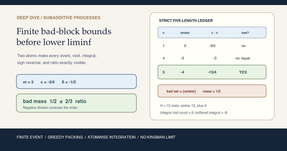
\[ m=5, \qquad c=-\frac34. \]A block of length \(n\) is bad at \(\omega\) when
\[ 1\le n\le5 \quad\text{and}\quad Y_n(\omega)\lt cn. \]Here is the complete finite search:
| \(n\) | \(Y_n(\text{amber})\) | \(cn\) | Amber is strictly bad? | Blue is strictly bad? |
|---|---|---|---|---|
| 1 | \(0\) | \(-3/4\) | no | no |
| 2 | \(-1\) | \(-3/2\) | no | no |
| 3 | \(-2\) | \(-9/4\) | no | no |
| 4 | \(-3\) | \(-3\) | no: equality is excluded | no |
| 5 | \(-4\) | \(-15/4\) | yes | no |
Write
\[ E_n(c)=\{\omega:Y_n(\omega)\lt cn\}. \]The rows give
\[ E_1=E_2=E_3=E_4=\varnothing, \qquad E_5=\{\text{amber}\}. \]The finite bad-block event is their union:
\[ \begin{aligned} B_5(-3/4) &=\bigcup_{n=1}^{5}E_n(-3/4)\\ &=\{\text{amber}\}. \end{aligned} \]Its exact probability is
\[ q:=\mu(B_5(-3/4))=\frac12. \]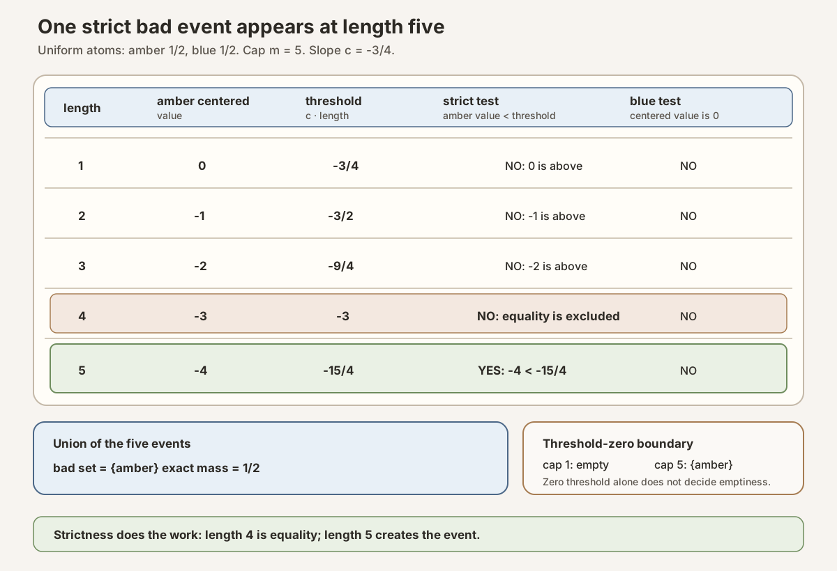
Two boundary tests before any theorem
If the cap is zero, there are no positive candidate lengths:
\[ B_0(c)=\varnothing \qquad\text{for every }c. \]Threshold zero needs more care. At cap one,
\[ B_1(0)=\varnothing \]because \(Y_1=0\) and the event uses a strict inequality. It is false that threshold zero always makes the bad event empty. With the same process and cap five,
\[ B_5(0)=\{\text{amber}\}, \]because \(Y_2(\text{amber})=-1\lt0\). The cap, strictness, and sign must all be read together.
Count twelve visits, then pack three witnesses
Choose a counting horizon
\[ H=12. \]The finite orbit-visit count is
\[ N_H(\omega) := \#\{j\in\{0,\ldots,H-1\}:T^j\omega\in B_5(-3/4)\}. \]The amber orbit remains in the bad event at all twelve starts, while the blue orbit never enters it:
\[ N_{12}(\text{amber})=12, \qquad N_{12}(\text{blue})=0. \]At each marked amber start, length five is a witness because
\[ Y_5(\text{amber})=-4 \lt -\frac34\cdot5=-\frac{15}{4}. \]Starting from the left, a greedy disjoint cover can retain
\[ [0,5),\qquad[5,10),\qquad[10,15). \]These three intervals cover every marked start \(0,\ldots,11\). Their total covered length is \(15\), and they fit in the safe buffered horizon
\[ H+m=12+5=17. \]The selected interval costs add to
\[ -4-4-4=-12. \]The full amber chain is therefore
\[ \begin{aligned} Y_{17}(\text{amber}) &=-16\\ &\le -12\\ &\lt -\frac34\cdot15=-\frac{45}{4}\\ &\le -\frac34\cdot12=-9. \end{aligned} \]The final comparison uses both \(15\ge12\) and \(c\le0\). Multiplication by a nonpositive coefficient reverses the usual length comparison. The blue orbit has no marks and gives \(Y_{17}(\text{blue})=0\le0\).
Thus both atoms satisfy the pointwise theorem’s conclusion:
\[ Y_{H+m}(\omega)\le cN_H(\omega). \]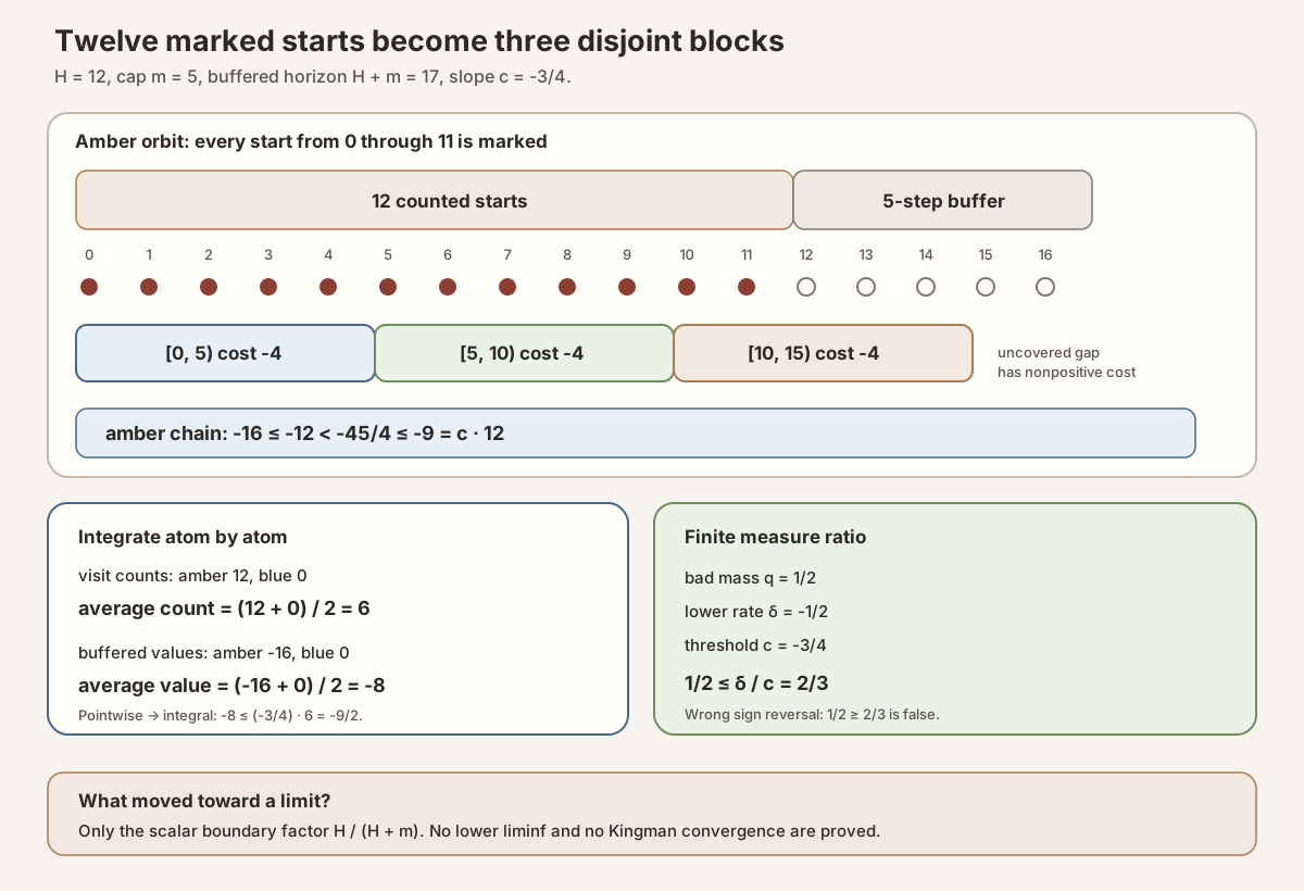
Integrate atom by atom
On this two-atom probability space, integrating a function means averaging its two values. For the visit count,
\[ \begin{aligned} \int_\Omega N_{12}\,d\mu &=\frac12\cdot12+\frac12\cdot0\\ &=6\\ &=12\cdot\mu(B_5(-3/4)). \end{aligned} \]This is the finite identity
\[ \int_\Omega N_H\,d\mu =H\,\mu(B_m(c)) \]made completely explicit.
For the buffered centered process,
\[ \int_\Omega Y_{17}\,d\mu =\frac12(-16)+\frac12(0) =-8. \]The integrated right side is
\[ c\int_\Omega N_{12}\,d\mu =-\frac34\cdot6 =-\frac92. \]The pointwise inequality therefore integrates to the true finite comparison
\[ -8\le-\frac92. \]Nothing was averaged over time here. We integrated two finite atom values after proving a finite pointwise inequality.
Compute the lower-rate witness and the ratio
Let
\[ I_n:=\int_\Omega Y_n\,d\mu. \]For every positive \(n\),
\[ I_n=-\frac{n-1}{2}. \]Consequently,
\[ \frac{I_n}{n} =-\frac12+\frac{1}{2n} \ge-\frac12. \]Choose
\[ \delta=-\frac12. \]This is a lower bound for every positive normalized centered integral. It is not a statement about samplewise convergence. It is one deterministic inequality for the scalar sequence \(I_n/n\).
At the displayed buffered horizon,
\[ \delta(H+m) =-\frac12\cdot17 =-\frac{17}{2} \le I_{17}=-8 \le cHq=-\frac92. \]For an arbitrary positive \(H\), the same proof gives
\[ \delta \le cq\frac{H}{H+m}. \]Only the elementary scalar factor moves toward a limit:
\[ \frac{H}{H+m}\longrightarrow1. \]Hence
\[ \delta\le cq. \]Because
\[ c=-\frac34\lt-\frac12=\delta\le0, \]division by \(c\) reverses the inequality:
\[ q\le\frac{\delta}{c}. \]In the running example,
\[ \boxed{\frac12\le \frac{-1/2}{-3/4} =\frac23.} \]This is the requested finite measure ratio.
The sign-reversal near miss
If one divides \(\delta\le cq\) by the negative number \(c\) without reversing the order, one obtains the wrong proposal
\[ q\ge\frac{\delta}{c}. \]Our exact values refute it:
\[ \frac12\not\ge\frac23. \]This error is not a minor notation issue. It changes a useful upper bound into a false lower bound.
Climb from the finite ledger to the general definitions
Now let \((\Omega,\mu)\) be any measurable space with finite total measure, let \(T:\Omega\to\Omega\) preserve \(\mu\), and let \(X_n:\Omega\to\mathbb R\) be an integrable shifted-subadditive process:
\[ X_{a+b}(\omega) \le X_b(T^a\omega)+X_a(\omega). \]Define the orbit-majorant-centered process
[ Y_n(\omega) := X_n(\omega)
\sum_{j=0}^{n-1}X_1(T^j\omega). ]
The word centered here does not mean expectation centering. The subtracted quantity depends on \(\omega\). Shifted subadditivity gives
\[ Y_1=0, \qquad Y_n\le0\quad(n\gt0), \]and \(Y\) is again shifted subadditive.
In Lean: define the finite strict bad-block event
finiteCenteredBadBlockSet T X m cfiniteCenteredBadBlockSetis aSet Ω, so it is an event, not a number.Finset.Icc 1 mis the inclusive finite window \(1\le n\le m\).⋃ n ∈ Finset.Icc 1 mforms the finite union over witness lengths.centeredProcess T X n ωis \(Y_n(\omega)\).< c * (n : ℝ)is strict and casts the natural length to a real number.- No probability, preservation, integrability, or ergodicity hypothesis is needed merely to define this set.
The exact source definition is:
def finiteCenteredBadBlockSet {Ω : Type uΩ} (T : Ω → Ω)
    (X : ℕ → Ω → ℝ) (m : ℕ) (c : ℝ) : Set Ω :=
  ⋃ n ∈ Finset.Icc 1 m,
    {ω | centeredProcess T X n ω < c * (n : ℝ)}
Candidate integrability and preservation are introduced only when the source proves that this finite union is null measurable. A null set has measure zero. A null measurable set may differ from an ordinary measurable set by a null set. That weaker regularity is exactly what the integration interface needs.
Turn visits into an indicator Birkhoff sum
For a set \(s\subseteq\Omega\), define
\[ N_H^s(\omega) := \#\{j\in\{0,\ldots,H-1\}:T^j\omega\in s\}. \]The corresponding Birkhoff sum is finite:
\[ \sum_{j=0}^{H-1}\mathbf 1_s(T^j\omega). \]The symbol \(\mathbf 1_s\) is the indicator of \(s\): it is one on \(s\) and zero outside.
In Lean: cast the count to the exact finite sum
natCast_finiteOrbitVisitCount_eq_birkhoffSum_indicator T s H ωfiniteOrbitVisitCount T s H ωis a natural-number cardinality.( ... : ℝ)is its real cast.birkhoffSum Tsamples along iterates of the original map \(T\).s.indicator fun _ ↦ (1 : ℝ)is the real-valued indicator.His the exact number of summands.- This theorem is finite combinatorics. It assumes no measurable space, measure, preservation, probability, or ergodicity.
At \(H=0\), both sides are zero. No separate positivity premise is required.
In Lean: integrate the finite visit count
integral_finiteOrbitVisitCount hT hs H[IsFiniteMeasure μ]says the whole space has finite total mass.hT : MeasurePreserving T μ μkeeps \(\mu\) unchanged under \(T\).hs : NullMeasurableSet s μis enough for indicator integration.μ.real sis Mathlib’s real-valued projection of the measure of \(s\).H * μ.real suses the coerced natural horizon as a real scalar.- The conclusion is exact for every finite \(H\), including zero.
Probability normalization is absent. If the total mass were two, the two sides would both scale by two.
From one witness per visit to a pointwise cost bound
At every marked start \(j\lt H\), membership in \(B_m(c)\) supplies at least one witness length
\[ 1\le\ell(j)\le m, \qquad Y_{\ell(j)}(T^j\omega)\lt c\ell(j). \]The source uses classical choice to select one such \(\ell(j)\). It does not choose a shortest, longest, or globally optimal witness. RMT-21’s greedy interval theorem then extracts disjoint intervals that cover every marked start.
Positive-time nonpositivity lets the proof discard uncovered gaps from an upper bound. Shifted subadditivity concatenates the retained interval costs. Because \(c\le0\), covered length at least the number of marks implies the marked-cardinality estimate in the required direction.
In Lean: obtain the buffered pointwise inequality
hX.centeredProcess_le_badBlockVisitCount H m hHm c hc ωhXpackages finite-horizon integrability and shifted subadditivity.hHm : H + m ≠ 0excludes the genuine joint zero corner.hc : c ≤ 0is needed when covered length is compared with marked cardinality.ωremains arbitrary, so the result is pointwise.- The proof body consumes shifted subadditivity and positive-time nonpositivity. The public receiver still carries the stronger integrability package.
- No measure, probability, preservation, ergodicity, or limit appears in the conclusion.
The corner \(H=m=0\) cannot be erased. Then the right side is zero while
\[ Y_0=X_0 \]may be positive. If \(H=0\) but \(m\gt0\), the theorem reduces to \(Y_m\le0\), which is valid. If \(m=0\) but \(H\gt0\), the bad set is empty and the theorem reduces to \(Y_H\le0\).
Integrate first, then remove only the finite buffer
Assume a scalar \(\delta\) satisfies
\[ \delta \le \frac{\int_\Omega Y_n\,d\mu}{n} \qquad \text{for every }n\gt0. \]Applying this at \(H+m\), integrating the pointwise packing bound, and using the exact count identity gives
\[ \delta \le \left(c\,\mu_{\mathbb R}(B_m(c))\right) \frac{H}{H+m}. \]At time one, \(Y_1=0\), so the premise forces \(\delta\le0\). The additional assumption \(c\lt\delta\) gives \(c\lt0\). The elementary coefficient tends to one as \(H\) grows. Therefore
\[ \delta \le c\,\mu_{\mathbb R}(B_m(c)). \]Negative division finally yields the finite ratio.
In Lean: invoke the generic finite-measure ratio
hX.measureReal_finiteCenteredBadBlockSet_le_rateRatio hT m δ c hδ hc[IsFiniteMeasure μ]is the only total-mass typeclass.hTsupplies preservation of \(\mu\) by \(T\).hδhas type∀ n : ℕ, n ≠ 0 → δ ≤ (∫ ω, centeredProcess T X n ω ∂μ) / (n : ℝ).hc : c < δlets the proof derive both \(\delta\le0\) and \(c\lt0\).le_div_iff_of_neg hcnegperforms the final order reversal explicitly.- The theorem contains no probability or ergodicity premise.
- The only limiting object is the deterministic coefficient \(H/(H+m)\), not a sample process.
The stronger strict comparison \(c\lt\delta\) also makes
\[ 0\le\frac{\delta}{c}\lt1. \]That subunit ceiling is useful to a later probability-and-ergodicity argument. This module does not perform that later argument.
Specialize the lower-rate witness to matrix cocycles
For a discrete matrix cocycle \(C\), let
\[ \begin{aligned} X_n(\omega) &=\log^+\lVert C(n,\omega)\rVert_\infty. \end{aligned} \]The one-step log-positive integrability package produces an integrable subadditive candidate. Define the deterministic offset
[ \delta_C := \gamma_\mu^+(C)
\int_\Omega X_1,d\mu, ]
where \(\gamma_\mu^+(C)\) is the integrated log-positive Fekete rate.
In Lean: prove the cocycle offset is a lower bound
hC.centeredFeketeOffset_le_normalizedIntegral n hnhC : C.HasIntegrableGeneratorLogPlussupplies one-step integrability.n : ℕis the finite horizon.hn : n ≠ 0licenses real division by the cast horizon.integratedLogPlusGrowthRate hCis a deterministic infimum from Fekete’s lemma.integratedLogPlusNorm 1is the raw one-step integral.integral_centeredProcessrewrites the centered integral exactly.- This theorem compares deterministic integrals. It is not a samplewise limit.
In Lean: obtain the cocycle finite bad-set ratio
hC.measureReal_centeredLogPlusBadBlockSet_le_rateRatio m c hccenteredLogPlusBadBlockSetis only a named specialization of the generic event.[IsFiniteMeasure μ]supplies finite total mass.C.base_preservingsupplies preservation already bundled with the cocycle.hC.isIntegrableSubadditiveProcessCandidatesupplies the generic process.hcis the strict threshold comparison.- No
PreErgodic,Ergodic,IsProbabilityMeasure, or nonempty matrix-index hypothesis is introduced. - The endpoint remains valid when the finite matrix index type is empty.
Assumption ledger: keep the layers separate
| Layer | Assumptions actually exposed | What it obtains |
|---|---|---|
| Define \(B_m(c)\) | A map \(T\), process \(X\), cap \(m\), slope \(c\) | A set of sample points |
| Count visits | A map, set, finite horizon, sample point | A natural number |
| Cast count to a Birkhoff sum | Finite combinatorics only | Exact pointwise equality |
| Prove bad-set regularity | Candidate integrability and measure preservation | Null measurability |
| Pack witnesses pointwise | Shifted subadditivity, positive-time nonpositivity, \(H+m\ne0\), \(c\le0\) | \(Y_{H+m}\le cN_H\) |
| Integrate visit counts | Finite total measure, preservation, null measurability | \(\int N_H=H\mu_{\mathbb R}(B)\) |
| Prove the generic ratio | All preceding measure hypotheses, the all-positive-horizon lower bound, \(c\lt\delta\) | \(\mu_{\mathbb R}(B_m(c))\le\delta/c\) |
| Specialize to cocycles | Finite total measure and integrable generator log-positive norm | The same finite ratio for \(B_m^C(c)\) |
The opening example uses a probability measure to make atomwise averaging explicit. The generic theorem needs only a finite measure. Neither the generic theorem nor its cocycle specialization needs ergodicity.
Exact declaration map
The source exposes ten public declarations in dependency order:
| # | Public declaration | Exact role |
|---|---|---|
| 1 | finiteOrbitVisitCount | Defines the natural count of visits among positions \(0,\ldots,H-1\) |
| 2 | natCast_finiteOrbitVisitCount_eq_birkhoffSum_indicator | Casts that count to the exact indicator Birkhoff sum |
| 3 | integral_finiteOrbitVisitCount | Integrates the count as \(H\mu_{\mathbb R}(s)\) |
| 4 | finiteCenteredBadBlockSet | Defines the strict finite union over Finset.Icc 1 m |
| 5 | IsIntegrableSubadditiveProcessCandidate.nullMeasurableSet_finiteCenteredBadBlockSet | Proves null measurability under preservation |
| 6 | IsIntegrableSubadditiveProcessCandidate.centeredProcess_le_badBlockVisitCount | Proves the buffered pointwise packing bound |
| 7 | IsIntegrableSubadditiveProcessCandidate.measureReal_finiteCenteredBadBlockSet_le_rateRatio | Proves the generic finite-measure ratio |
| 8 | DiscreteMatrixCocycle.centeredLogPlusBadBlockSet | Names the cocycle’s finite centered bad-block event |
| 9 | DiscreteMatrixCocycle.HasIntegrableGeneratorLogPlus.centeredFeketeOffset_le_normalizedIntegral | Supplies the normalized-centered-integral lower bound |
| 10 | DiscreteMatrixCocycle.HasIntegrableGeneratorLogPlus.measureReal_centeredLogPlusBadBlockSet_le_rateRatio | Specializes the generic ratio to the cocycle |
The previous version of this chapter counted nine and omitted declaration 9. The table above matches the checked 506-line source.
All eleven private support declarations
| Private item | Why it exists |
|---|---|
rmt30ZeroProcess | A process that is zero at every horizon and sample |
rmt30ZeroProcess_candidate | Packages that process as an integrable shifted-subadditive candidate |
rmt30PositiveAtZeroProcess | Makes only the time-zero value positive |
rmt30PositiveAtZeroProcess_candidate | Certifies the joint-zero countermodel as a valid candidate |
rmt30TwoPointProbability | Defines the equal-weight Bool probability measure |
Anonymous IsProbabilityMeasure rmt30TwoPointProbability instance | Checks that the two half masses sum to one |
rmt30Id_not_preErgodic | Proves the identity base is not pre-ergodic |
rmt30TwoPointProcess | Defines the exact amber/blue process used in this chapter |
rmt30TwoPointProcess_candidate | Certifies its integrability and shifted subadditivity |
rmt30MassTwoMeasure | Defines a finite measure of total mass two |
Anonymous IsFiniteMeasure rmt30MassTwoMeasure instance | Supplies the finite-mass typeclass for the rescaling boundary |
All nine compiled anonymous boundary examples
- A zero cap makes the candidate-length window empty.
- Horizon zero is valid when the cap is positive.
- The zero process has no bad blocks at a negative threshold.
- The joint corner \(H=m=0\) fails for the positive-at-zero candidate.
- Zero measure gives every bad set real measure zero.
- The nonergodic two-point identity model has exact bad mass \(1/2\) and satisfies \(1/2\le2/3\).
- Equality with the time-one zero threshold is not marked.
- A mass-two finite measure is accepted without probability normalization.
- The cocycle endpoint accepts an empty matrix-index type.
All seven axiom reports
The file prints axiom footprints for:
natCast_finiteOrbitVisitCount_eq_birkhoffSum_indicator;integral_finiteOrbitVisitCount;nullMeasurableSet_finiteCenteredBadBlockSet;centeredProcess_le_badBlockVisitCount;measureReal_finiteCenteredBadBlockSet_le_rateRatio;centeredFeketeOffset_le_normalizedIntegral; andmeasureReal_centeredLogPlusBadBlockSet_le_rateRatio.
The source’s recorded project validation found the expected Mathlib logical footprint.
A bounded executable model using only Std
The next worksheet reproduces the complete two-atom ledger without importing Mathlib or this project. It is a standalone tutorial suitable for a normal macOS or Linux machine. It is not a proof of the general measure theorem.
Save this exact block as
/tmp/SubadditiveBadBlockMeasureTutorial.lean:
import Std

namespace SubadditiveBadBlockMeasureTutorial

inductive Atom where
  | amber
  | blue
  deriving Repr, DecidableEq

open Atom

def cap : Nat := 5
def countingHorizon : Nat := 12
def bufferedHorizon : Nat := countingHorizon + cap
def slope : Rat := -(3 : Rat) / 4
def lowerRate : Rat := -(1 : Rat) / 2

def centered (n : Nat) : Atom → Rat
  | amber => -((n - 1 : Nat) : Rat)
  | blue => 0

def candidateLengths (m : Nat) : List Nat :=
  (List.range m).map Nat.succ

def badAtLength (c : Rat) (n : Nat) (ω : Atom) : Bool :=
  decide (centered n ω < c * (n : Rat))

def badAtCap (m : Nat) (c : Rat) (ω : Atom) : Bool :=
  (candidateLengths m).any fun n => badAtLength c n ω

def shortRows : List (Nat × Rat × Rat × Bool × Bool) :=
  (candidateLengths cap).map fun n =>
    (n, centered n amber, slope * (n : Rat),
      badAtLength slope n amber, badAtLength slope n blue)

def badSet : List Atom :=
  [amber, blue].filter fun ω => badAtCap cap slope ω

def visitCount (H : Nat) (ω : Atom) : Nat :=
  ((List.range H).filter fun _ => badAtCap cap slope ω).length

def packedStarts : List Nat := [0, 5, 10]

def packedIntervals : List (Nat × Nat) :=
  packedStarts.map fun start => (start, start + cap)

def allMarkedStartsCovered : Bool :=
  (List.range countingHorizon).all fun j =>
    packedStarts.any fun start =>
      decide (start ≤ j ∧ j < start + cap)

def packedCost : Rat :=
  (packedStarts.map fun _ => centered cap amber).sum

def coveredLength : Nat :=
  packedStarts.length * cap

def integral (f : Atom → Rat) : Rat :=
  (f amber + f blue) / 2

def badMass : Rat :=
  ((badSet.length : Rat) / 2)

def visitIntegral : Rat :=
  integral fun ω => (visitCount countingHorizon ω : Rat)

def bufferedIntegral : Rat :=
  integral fun ω => centered bufferedHorizon ω

def packingChain : List Bool :=
  [decide (centered bufferedHorizon amber ≤ packedCost),
   decide (packedCost ≤ slope * (coveredLength : Rat)),
   decide (slope * (coveredLength : Rat) ≤
     slope * (visitCount countingHorizon amber : Rat))]

def ratio : Rat :=
  lowerRate / slope

def zeroThresholdBoundary : Bool × Bool × Bool :=
  (badAtCap 0 slope amber,
   badAtCap 1 0 amber,
   badAtCap cap 0 amber)

#eval shortRows
#eval badSet
#eval [visitCount countingHorizon amber, visitCount countingHorizon blue]
#eval packedIntervals
#eval (allMarkedStartsCovered, packedCost, coveredLength, packingChain)
#eval (visitIntegral,
  (countingHorizon : Rat) * badMass,
  bufferedIntegral,
  slope * visitIntegral)
#eval (badMass, ratio,
  decide (badMass ≤ ratio),
  decide (badMass ≥ ratio))
#eval zeroThresholdBoundary

example : shortRows =
    [(1, 0, -(3 : Rat) / 4, false, false),
     (2, -1, -(3 : Rat) / 2, false, false),
     (3, -2, -(9 : Rat) / 4, false, false),
     (4, -3, -3, false, false),
     (5, -4, -(15 : Rat) / 4, true, false)] := by
  native_decide

example : badSet = [amber] := by native_decide
example : packedIntervals = [(0, 5), (5, 10), (10, 15)] := by native_decide
example : allMarkedStartsCovered := by native_decide
example : packingChain = [true, true, true] := by native_decide
example : visitIntegral = 6 := by native_decide
example : bufferedIntegral = -8 := by native_decide
example : badMass = (1 : Rat) / 2 := by native_decide
example : ratio = (2 : Rat) / 3 := by native_decide
example : badMass ≤ ratio := by native_decide
example : ¬ badMass ≥ ratio := by native_decide
example : zeroThresholdBoundary = (false, false, true) := by native_decide

end SubadditiveBadBlockMeasureTutorial
Type:
source "$HOME/.elan/env"
elan run leanprover/lean4:v4.32.0 lean \
  /tmp/SubadditiveBadBlockMeasureTutorial.lean
The exact worksheet above was run successfully under Lean 4.32.0. Its exact transcript is:
[(1, 0, (-3 : Rat)/4, false, false),
 (2, -1, (-3 : Rat)/2, false, false),
 (3, -2, (-9 : Rat)/4, false, false),
 (4, -3, -3, false, false),
 (5, -4, (-15 : Rat)/4, true, false)]
[SubadditiveBadBlockMeasureTutorial.Atom.amber]
[12, 0]
[(0, 5), (5, 10), (10, 15)]
(true, -12, 15, [true, true, true])
(6, 6, -8, (-9 : Rat)/2)
((1 : Rat)/2, (2 : Rat)/3, true, false)
(false, false, true)
Read the last two lines carefully:
- the actual mass is \(1/2\);
- the ratio ceiling is \(2/3\);
truecertifies \(1/2\le2/3\);falserefutes the unreversed proposal \(1/2\ge2/3\); and- the final triple says cap zero is empty, cap one at threshold zero is empty, but cap five at threshold zero is not empty.
Inspect and check the exact project interfaces
The authoritative source is
formalization/NonlinearDynamics/Random/RandomCocycles/SubadditiveBadBlockMeasure.lean.
For a full project check, install the repository’s pinned dependencies and
place these inspection commands in a temporary project scratch file:
import NonlinearDynamics.Random.RandomCocycles.SubadditiveBadBlockMeasure

open MeasureTheory
open NonlinearDynamics.Random.RandomCocycles

#check finiteOrbitVisitCount
#check natCast_finiteOrbitVisitCount_eq_birkhoffSum_indicator
#check integral_finiteOrbitVisitCount
#check finiteCenteredBadBlockSet
#check IsIntegrableSubadditiveProcessCandidate.nullMeasurableSet_finiteCenteredBadBlockSet
#check IsIntegrableSubadditiveProcessCandidate.centeredProcess_le_badBlockVisitCount
#check IsIntegrableSubadditiveProcessCandidate.measureReal_finiteCenteredBadBlockSet_le_rateRatio
#check DiscreteMatrixCocycle.centeredLogPlusBadBlockSet
#check DiscreteMatrixCocycle.HasIntegrableGeneratorLogPlus.centeredFeketeOffset_le_normalizedIntegral
#check DiscreteMatrixCocycle.HasIntegrableGeneratorLogPlus.measureReal_centeredLogPlusBadBlockSet_le_rateRatio
The exact module check from the repository root is:
cd formalization
lake env lean NonlinearDynamics/Random/RandomCocycles/SubadditiveBadBlockMeasure.lean
That Mathlib-backed command may require substantial disk space and memory. The
lightweight Std worksheet above is the smaller learning path.
cd formalization
lake env lean -DwarningAsError=true NonlinearDynamics/Random/RandomCocycles/SubadditiveBadBlockMeasure.lean
Resource note: this exact file uses the repository's
pinned Lean and Mathlib dependencies. Initial project setup can require
substantial disk space and build time. For a lightweight first step on
macOS or Linux, use the page's standalone Lean-core or Std
tutorial.
Neither command changes pro_reviewed: false; technical validation and human
review are separate gates.
Common wrong turns
Treating the bad event as a long-time event
\(B_m(c)\) asks whether one witness exists among finitely many lengths. It does not mean:
- bad blocks occur infinitely often;
- witnesses occur after every cutoff;
- a normalized lower limit is below \(c\); or
- the process converges.
Those are different events with different quantifiers.
Replacing strict inequality by a weak one
At length four in the running example,
\[ Y_4(\text{amber})=-3=c\cdot4. \]The block is not marked. Replacing \(\lt\) by \(\le\) changes the event.
Forgetting the orbit shift
At a marked start \(j\), the witness cost is
\[ Y_{\ell(j)}(T^j\omega), \]not \(Y_{\ell(j)}(\omega)\) unless the base happens to be the identity. The running example uses identity dynamics for arithmetic clarity. The theorem does not.
Calling the pointwise packing theorem measure theoretic
The public method is attached to an integrable candidate, but its proof body uses shifted subadditivity and positive-time nonpositivity. The integration field is consumed later, when the inequality is integrated.
Calling a finite measure a probability measure
The generic theorem assumes finite total mass, not total mass one. The source compiles a mass-two boundary. Probability normalization becomes important only when a later argument interprets a strict subunit ratio canonically.
Claiming that the auxiliary limit is Kingman’s theorem
The proof sends the elementary number \(H/(H+m)\) to one. It does not prove that \(Y_n(\omega)/n\), \(X_n(\omega)/n\), or any matrix growth observable converges.
What this module proves
It proves:
- a natural-valued finite orbit-visit count;
- the exact equality between its real cast and an indicator Birkhoff sum;
- exact finite visit-count integration under finite measure and preservation;
- null measurability of the finite centered strict bad-block event;
- a pointwise greedy-packing estimate on the buffered horizon;
- a generic finite-measure ratio with negative division made explicit;
- the integrated Fekete-offset lower-bound bridge; and
- the finite log-positive matrix-cocycle specialization.
It proves neither lower liminf nor Kingman convergence. It also proves no:
- almost-everywhere convergence;
- equality of a sample rate with the integrated Fekete rate;
- \(L^1\) convergence;
- limit-integral interchange;
- ergodicity of \(T\) or a powered map;
- signed logarithmic growth theorem;
- Lyapunov exponent;
- Oseledets filtration or splitting; or
- quantitative rate or concentration inequality.
The next chapters first pass from fixed finite caps to the union over all positive lengths, then build an arbitrarily-late rational-threshold event. Only later does an ergodic probability argument connect such events to a lower liminf.
Exercises with answers
- Which candidate length is bad on amber? Only \(n=5\). At \(n=4\) the value equals the threshold, and strictness excludes it.
- What is the bad event? \(B_5(-3/4)=\{\text{amber}\}\).
- What is its probability? \(1/2\).
- Why does blue contribute no visits? Its orbit remains blue and every centered value is zero, while all five thresholds are negative.
- Why do twelve amber marks need only three retained intervals? The intervals \([0,5)\), \([5,10)\), and \([10,15)\) cover all starts \(0,\ldots,11\).
- What is their total cost? Three copies of \(-4\), hence \(-12\).
- Why is \(-45/4\le-9\)? Covered length \(15\) is at least marked count \(12\), and multiplying by \(-3/4\) reverses the comparison.
- Compute the visit integral. \((12+0)/2=6\).
- Compute the buffered-process integral. \((-16+0)/2=-8\).
- Why is \(\delta=-1/2\) valid for every positive \(n\)? Because \(I_n/n=-1/2+1/(2n)\ge-1/2\).
- Compute the theorem’s ceiling. \(\delta/c=(-1/2)/(-3/4)=2/3\).
- What does the wrong sign rule predict? \(1/2\ge2/3\), which is false.
- Is \(B_1(0)\) empty? Yes, because \(Y_1=0\) and the test is strict.
- Is \(B_5(0)\) empty in this model? No. Amber is already bad at length two.
- Where is probability normalization used in the generic theorem? Nowhere. The example uses it for a simple atomwise calculation.
- Where is ergodicity used? Nowhere in this module.
- What limit is taken? Only \(H/(H+m)\to1\) for fixed \(m\).
- What major theorem is still absent? Any lower-liminf conclusion and Kingman’s samplewise convergence theorem.
Continue the dependency-ordered climb
The immediate predecessor is Finite Ordered Interval Packing for Nonpositive Subadditive Processes. The next textbook step is From Finite Centered Bad-Block Bounds to All-Positive-Length Control. The paired Development Notebook records the proof construction and source history. The finite orbit-visit count glossary chapter isolates the counting primitive.
References
J. F. C. Kingman. The ergodic theory of subadditive stochastic processes, Journal of the Royal Statistical Society: Series B 30(3), 499-510, 1968, doi:10.1111/j.2517-6161.1968.tb00749.x. This is the primary source for the full theorem that this finite module does not yet prove.
J. Michael Steele. Kingman’s subadditive ergodic theorem, Annales de l’Institut Henri Poincare, Probabilites et Statistiques 25(1), 93-98, 1989. Steele gives an interval-decomposition proof of the full theorem. RMT-30 isolates and checks one finite bad-block measure bridge from that proof lineage.
Mathlib contributors.
Indicator integration,
Mathlib commit 81a5d257. The pinned library supplies the null-measurable
indicator integration interface used by the checked proof.
Mathlib contributors.
Elementary limits at infinity,
Mathlib commit 81a5d257. The source uses
tendsto_natCast_div_add_atTop only for the auxiliary finite-buffer
coefficient.
The audited Lean source SHA-256 for this chapter is
a8aee618a10f8434c1c33d8e433fd77e98ed3e5c8dee399e7d6fa323c5079b28.