Finite GUE Empirical Spectral Laws and Normalized Moments

Start with two matrices you can completely see

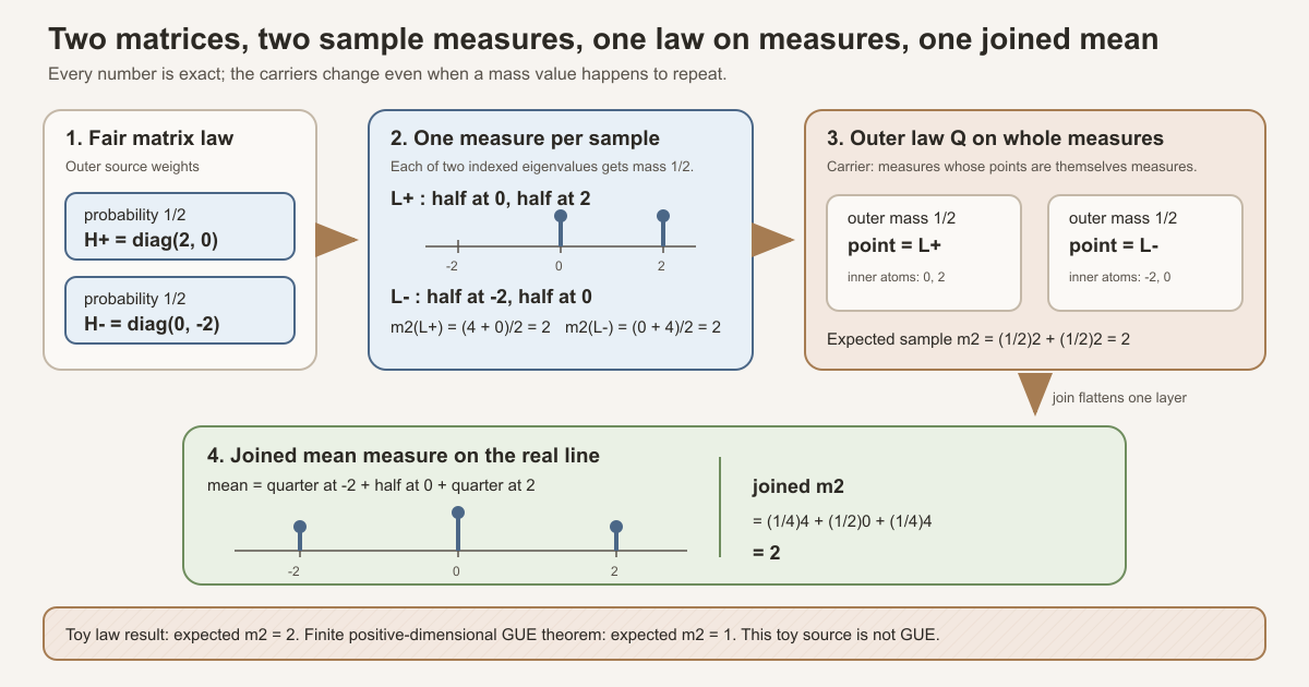
A probability law assigns mass to measurable subsets of a value space. In this first finite example it has two atoms, both \(2\)-by-\(2\) real diagonal matrices and therefore complex Hermitian matrices :

\[ H_+= \begin{bmatrix} 2&0\\ 0&0 \end{bmatrix}, \qquad H_-= \begin{bmatrix} 0&0\\ 0&-2 \end{bmatrix}. \]

A fair source chooses each matrix with probability \(1/2\). Call this matrix law \(P\):

\[ P=\frac12\delta_{H_+}+\frac12\delta_{H_-}. \]

Here \(\delta_a\) is the Dirac measure at \(a\): it puts all of its mass at the one point \(a\). The sample space of \(P\) is a two-point set of matrices. There is no Gaussian distribution in this example.

The eigenvalues are visible on the diagonals:

\[ \operatorname{spec}(H_+)=\{2,0\}, \qquad \operatorname{spec}(H_-)=\{0,-2\}. \]

Each list has two indexed eigenvalues. The empirical spectral measure assigns mass \(1/2\) to each indexed eigenvalue:

\[ L_+=\frac12\delta_2+\frac12\delta_0, \qquad L_-=\frac12\delta_0+\frac12\delta_{-2}. \]

Both \(L_+\) and \(L_-\) are probability measures on the real line: their total mass is one.

Put a law on the whole sample measures

The map

\[ H\longmapsto L_H \]

turns a matrix outcome into a measure outcome. Pushing the matrix law through that map gives the empirical spectral law

\[ Q=\frac12\delta_{L_+}+\frac12\delta_{L_-}. \]

This time the points carrying outer mass are \(L_+\) and \(L_-\), not the real numbers \(2,0,-2\). The type has changed:

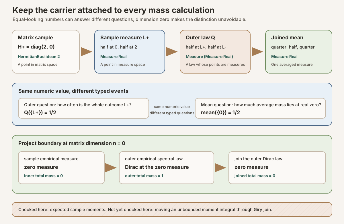
\[ L_\pm\in\operatorname{Measure}(\mathbb R), \qquad Q\in\operatorname{Measure}(\operatorname{Measure}(\mathbb R)). \]

For example,

\[ Q(\{L_+\})=\frac12. \]

That statement asks how often the whole measure \(L_+\) occurs.

Join the law to obtain one mean measure

Mathlib’s Giry join operation averages the measure-valued outcomes of a measure on measures. In this finite example it means: multiply every inner atom by its outer probability, then collect equal real locations.

The \(H_+\) branch contributes

\[ \frac12L_+=\frac14\delta_2+\frac14\delta_0, \]

and the \(H_-\) branch contributes

\[ \frac12L_-=\frac14\delta_0+\frac14\delta_{-2}. \]

Adding the branches gives the joined mean measure

\[ \overline L=\operatorname{join}(Q) =\frac14\delta_2+\frac12\delta_0+\frac14\delta_{-2}. \]

Now

\[ \overline L(\{0\})=\frac12. \]

The number \(1/2\) happens to match \(Q(\{L_+\})\), but the questions and carriers differ. The first evaluates a law on a set of measures. The second evaluates a measure on a set of real numbers.

Compute a normalized spectral moment

For a sample empirical measure \(L_H\), define its \(k\)-th spectral moment by

\[ m_k(H)=\int_{\mathbb R}x^k\,\mathrm dL_H(x). \]

Because the empirical measure already divides the counting mass by matrix dimension, this is the normalized spectral moment. For the second moment:

\[ \begin{aligned} m_2(H_+)&=\frac12(2^2)+\frac12(0^2)=2,\\ m_2(H_-)&=\frac12(0^2)+\frac12((-2)^2)=2. \end{aligned} \]

The expectation across the outer matrix law is therefore

\[ \mathbb E_P[m_2(H)]=\frac12(2)+\frac12(2)=2. \]

Direct finite enumeration also gives

\[ \int x^2\,\mathrm d\overline L(x) =\frac14(2^2)+\frac12(0^2)+\frac14((-2)^2)=2. \]

That final equality is proved here only for this finite toy source by expanding four terms. It is not the general moment-through-join theorem that the project would need for unbounded complex-valued integrands.

A fair source chooses the diagonal matrix with entries two and zero or the diagonal matrix with entries zero and minus two. Their empirical spectral measures receive outer mass one half each. Joining gives one quarter mass at minus two, one half at zero, and one quarter at two. The toy expected second moment is exactly two. — FigureFinding: the fair matrix law has two matrix outcomes. The empirical-measure map sends them to \(L_+=\tfrac12\delta_2+\tfrac12\delta_0\) and \(L_-=\tfrac12\delta_0+\tfrac12\delta_{-2}\). The outer law \(Q=\tfrac12\delta_{L_+}+\tfrac12\delta_{L_-}\) therefore has whole measures as points. Giry join flattens one layer and gives \(\overline L=\tfrac14\delta_2+\tfrac12\delta_0+\tfrac14\delta_{-2}\). Both sample second moments, their outer expectation, and the directly enumerated second moment of this finite joined mean equal \(2\). This source is a teaching model, not the Gaussian unitary ensemble; the checked positive-dimensional GUE expectation later in the chapter is \(1\).

Three nearby wrong turns

Treating \(Q\) as a measure on real numbers. The expression \(Q(\{2\})\) is ill-typed. A point of \(Q\)’s carrier is a measure such as \(L_+\), not a real eigenvalue such as \(2\).
Treating the join as an inverse. From \(\overline L\) alone one cannot recover whether the mass at \(2\) and the mass at \(-2\) occurred in different trials, the same trial, or a more complicated mixture. Join loses fluctuations of whole measures.
Calling the toy law GUE. The Gaussian unitary ensemble (GUE) is a Gaussian law on finite Hermitian matrices with the project’s specified variance normalization. In positive dimension it has a continuous Gaussian coordinate presentation; at size zero it is degenerate. A fair law on two diagonal matrices is not GUE merely because both laws are Hermitian and centered.

A matrix sample, its empirical measure, the outer law on measures, and the joined mean occupy four distinct carriers. In dimension zero the sample empirical measure has total mass zero, its outer Dirac law has total mass one, and joining returns the zero measure. — FigureFinding: \(H_+\), \(L_+\), \(Q\), and \(\overline L\) live respectively in matrix space, \(\operatorname{Measure}(\mathbb R)\), \(\operatorname{Measure}(\operatorname{Measure}(\mathbb R))\), and again \(\operatorname{Measure}(\mathbb R)\). In the toy model, \(Q(\{L_+\})\) and \(\overline L(\{0\})\) both equal \(1/2\), but the equal values do not erase the carrier distinction. At project dimension zero the inner empirical measure is the zero measure of total mass zero; the outer empirical spectral law is the mass-one Dirac law concentrated at that zero measure; joining returns the zero measure. The checked RMT-10C moment theorems integrate sample moments across matrices and do not yet move unbounded moments through join.

Type and run the complete finite ledger

The full GUE law, eigenvalue measurability, Giry join, and Bochner integrals are full project checks that use Mathlib and may require substantial disk space and memory. The finite two-outcome arithmetic is a standalone tutorial that can run on an ordinary macOS or Linux machine using only Lean’s standard library Std.

Create /tmp/GUESpectralLaw2Tutorial.lean and type:

import Std

structure DiagonalMatrix2 where
  upper : Int
  lower : Int
deriving Repr, DecidableEq

structure Atom where
  location : Int
  mass : Rat
deriving Repr, DecidableEq

structure AtomicMeasure where
  name : String
  atoms : List Atom
deriving Repr, DecidableEq

structure FiniteLaw (α : Type) where
  outcomes : List (α × Rat)
deriving Repr

def half : Rat := (1 : Rat) / 2
def quarter : Rat := (1 : Rat) / 4

def matrixPlus : DiagonalMatrix2 := ⟨2, 0⟩
def matrixMinus : DiagonalMatrix2 := ⟨0, -2⟩

def matrixLaw : FiniteLaw DiagonalMatrix2 :=
  ⟨[(matrixPlus, half), (matrixMinus, half)]⟩

def empiricalMeasure (H : DiagonalMatrix2) : AtomicMeasure :=
  ⟨s!"L({H.upper},{H.lower})",
    [⟨H.upper, half⟩, ⟨H.lower, half⟩]⟩

def FiniteLaw.map (f : α → β) (law : FiniteLaw α) : FiniteLaw β :=
  ⟨law.outcomes.map (fun pair => (f pair.1, pair.2))⟩

def empiricalSpectralLaw : FiniteLaw AtomicMeasure :=
  matrixLaw.map empiricalMeasure

def totalMass (μ : AtomicMeasure) : Rat :=
  (μ.atoms.map Atom.mass).sum

def lawMass (law : FiniteLaw α) : Rat :=
  (law.outcomes.map Prod.snd).sum

def massAt (μ : AtomicMeasure) (x : Int) : Rat :=
  (μ.atoms.filterMap fun atom =>
    if atom.location = x then some atom.mass else none).sum

def normalizedMoment (k : Nat) (μ : AtomicMeasure) : Rat :=
  (μ.atoms.map fun atom => atom.mass * (atom.location : Rat) ^ k).sum

def expectedMoment (k : Nat) (law : FiniteLaw AtomicMeasure) : Rat :=
  (law.outcomes.map fun pair =>
    pair.2 * normalizedMoment k pair.1).sum

def rawJoinedAtoms (law : FiniteLaw AtomicMeasure) : List Atom :=
  law.outcomes.flatMap fun pair =>
    pair.1.atoms.map fun atom => ⟨atom.location, pair.2 * atom.mass⟩

def rawJoinedMassAt (law : FiniteLaw AtomicMeasure) (x : Int) : Rat :=
  ((rawJoinedAtoms law).filterMap fun atom =>
    if atom.location = x then some atom.mass else none).sum

def joinedMean : AtomicMeasure :=
  ⟨"mean", [⟨-2, quarter⟩, ⟨0, half⟩, ⟨2, quarter⟩]⟩

def emptyEmpiricalMeasure : AtomicMeasure := ⟨"zero measure", []⟩

def emptyEmpiricalLaw : FiniteLaw AtomicMeasure :=
  ⟨[(emptyEmpiricalMeasure, 1)]⟩

#eval matrixLaw
#eval empiricalMeasure matrixPlus
#eval empiricalMeasure matrixMinus
#eval empiricalSpectralLaw.outcomes.map (fun pair => (pair.1.name, pair.2))
#eval [rawJoinedMassAt empiricalSpectralLaw (-2),
  rawJoinedMassAt empiricalSpectralLaw 0,
  rawJoinedMassAt empiricalSpectralLaw 2]
#eval [normalizedMoment 1 (empiricalMeasure matrixPlus),
  normalizedMoment 1 (empiricalMeasure matrixMinus),
  expectedMoment 1 empiricalSpectralLaw]
#eval [normalizedMoment 2 (empiricalMeasure matrixPlus),
  normalizedMoment 2 (empiricalMeasure matrixMinus),
  expectedMoment 2 empiricalSpectralLaw,
  normalizedMoment 2 joinedMean]
#eval (totalMass emptyEmpiricalMeasure, lawMass emptyEmpiricalLaw)

example : empiricalMeasure matrixPlus =
    ⟨"L(2,0)", [⟨2, half⟩, ⟨0, half⟩]⟩ := by
  native_decide

example : empiricalMeasure matrixMinus =
    ⟨"L(0,-2)", [⟨0, half⟩, ⟨-2, half⟩]⟩ := by
  native_decide

example : lawMass matrixLaw = 1 := by
  native_decide

example : lawMass empiricalSpectralLaw = 1 := by
  native_decide

example : rawJoinedMassAt empiricalSpectralLaw (-2) = quarter := by
  native_decide

example : rawJoinedMassAt empiricalSpectralLaw 0 = half := by
  native_decide

example : rawJoinedMassAt empiricalSpectralLaw 2 = quarter := by
  native_decide

example : normalizedMoment 1 (empiricalMeasure matrixPlus) = 1 := by
  native_decide

example : normalizedMoment 1 (empiricalMeasure matrixMinus) = -1 := by
  native_decide

example : expectedMoment 1 empiricalSpectralLaw = 0 := by
  native_decide

example : normalizedMoment 2 (empiricalMeasure matrixPlus) = 2 := by
  native_decide

example : normalizedMoment 2 (empiricalMeasure matrixMinus) = 2 := by
  native_decide

example : expectedMoment 2 empiricalSpectralLaw = 2 := by
  native_decide

example : normalizedMoment 2 joinedMean = 2 := by
  native_decide

example : totalMass emptyEmpiricalMeasure = 0 := by
  native_decide

example : lawMass emptyEmpiricalLaw = 1 := by
  native_decide

Run the pinned compiler directly:

source "$HOME/.elan/env"
elan run leanprover/lean4:v4.32.0 lean /tmp/GUESpectralLaw2Tutorial.lean

Resource label: small standalone Lean plus Std, suitable for an ordinary macOS or Linux machine. This command does not enter the Lake project, import Mathlib, or compile the formalization.

The executed output is:

{ outcomes := [({ upper := 2, lower := 0 }, (1 : Rat)/2), ({ upper := 0, lower := -2 }, (1 : Rat)/2)] }
{ name := "L(2,0)", atoms := [{ location := 2, mass := (1 : Rat)/2 }, { location := 0, mass := (1 : Rat)/2 }] }
{ name := "L(0,-2)", atoms := [{ location := 0, mass := (1 : Rat)/2 }, { location := -2, mass := (1 : Rat)/2 }] }
[("L(2,0)", (1 : Rat)/2), ("L(0,-2)", (1 : Rat)/2)]
[(1 : Rat)/4, (1 : Rat)/2, (1 : Rat)/4]
[1, -1, 0]
[2, 2, 2, 2]
(0, 1)

Read the last three lines carefully:

the joined masses at \(-2,0,2\) are \(1/4,1/2,1/4\);
the sample first moments are \(1,-1\), with outer expectation \(0\);
the two sample second moments, their outer expectation, and the explicitly enumerated joined second moment are all \(2\); and
the empty sample measure has total mass \(0\), while its one-point outer law has total mass \(1\).

The sixteen example declarations state the same rational equalities as propositions that Lean’s kernel checks. This worksheet represents finite atomic measures as lists. It does not construct the Giry measurable space, prove eigenvalue measurability, define GUE, prove Bochner integrability, or establish a general integration theorem for join.

From the finite ledger to RMT-10C

The project’s tenth random-matrix milestone, part C (RMT-10C), replaces each finite teaching structure with its genuine analytic object:

Teaching object	Project object	Exact carrier
`DiagonalMatrix2`	`HermitianEuclidean n`	Intrinsic finite Hermitian matrices
`AtomicMeasure`	`Measure ℝ`	Measures on the Borel real line
`FiniteLaw AtomicMeasure`	`Measure (Measure ℝ)`	Measures whose points are measures
outer law with mass-one evidence	`ProbabilityMeasure (Measure ℝ)`	Bundled outer probability law
positive-dimensional law with bundled outcomes	`ProbabilityMeasure (ProbabilityMeasure ℝ)`	Bundled law on bundled inner probabilities
explicit finite flattening	`Measure.join`	Giry join
rational list sum	complex Bochner integral	`ℂ`-valued integration

A measurable function is a function whose inverse images preserve the measurable sets needed by measure theory. That property lets Lean form a pushforward law. It is weaker than integrability , which additionally controls the size of an observable strongly enough for a genuine expectation.

RMT-10C consumes three earlier layers:

RMT-09 proves exact finite GUE trace integrability and expectations.
RMT-10A constructs ordered Hermitian eigenvalues, counting measures, and empirical spectral measures.
RMT-10B proves the eigenvalue and measure-valued maps measurable using a finite-dimensional Weyl perturbation bound.

RMT-10C then constructs the outer law, its probability packages, its joined mean, and the first two exact expected sample moments.

Type ledger: four uses of the word “average”

The same chapter contains four operations that a reader might casually call an average:

Operation	Input	Output	Toy value
Normalize eigenvalue atoms	Two indexed eigenvalues	One sample measure \(L_H\)	Half mass per eigenvalue
Average a scalar across matrix outcomes	\(m_k(H)\) and matrix law \(P\)	One scalar \(\mathbb E[m_k]\)	\(\mathbb E[m_2]=2\)
Average whole measures	Outer law \(Q\)	Joined measure \(\overline L\)	Quarter, half, quarter
Average \(x^k\) inside a measure	Measure and integrand	One scalar moment	\(\int x^2\,\mathrm d\overline L=2\) in the toy model

Only the first operation is built into the phrase empirical spectral measure. The next two integrate over different carriers. The fourth can be related to the third only through a suitable integration theorem.

Lean bridge one: one matrix produces one empirical measure

One idea, three languages Read across, then read the syntax map

A human says

Count every indexed Hermitian eigenvalue with multiplicity, then divide the counting measure by the matrix dimension. At dimension zero the project returns the zero measure.

On paper

\(N_H=\sum_{i\in\operatorname{Fin}(n)}\delta_{\lambda_i(H)},\qquad L_H=(n:\mathbb R_{\ge0}^{\infty})^{-1}N_H;\quad L_H=0\text{ when }n=0.\)

In Lean

RandomMatrix.empiricalSpectralMeasure H = (n : ℝ≥0∞)⁻¹ • RandomMatrix.spectralCountingMeasure H

Syntax map

H has type HermitianEuclidean n. Hermiticity is carried by the value rather than assumed later.
spectralCountingMeasure H is a Measure ℝ with one Dirac summand for each index in Fin n. Repeated eigenvalues retain multiplicity because repeated indices remain in the sum.
(n : ℝ≥0∞)⁻¹ is an inverse in the extended nonnegative reals, the scalar system used for measures.
• scales the entire measure.
The exact zero theorem is RandomMatrix.empiricalSpectralMeasure_zero; the positive-mass theorem is RandomMatrix.empiricalSpectralMeasure_succ_isProbability.

Try it in the repository. In the first full project probe below, import HermitianSpectrumContinuity, use #print on empiricalSpectralMeasure, and use #check on its zero and positive-dimensional theorems. The full project command checks the authoritative project leaf with its pinned dependencies.

Why the zero formula is not \(1/0\) handwaving

At \(n=0\), the finite index Fin 0 is empty, so the spectral counting measure is zero. The scalar inverse lives in \(\mathbb R_{\ge0}^{\infty}\), where the inverse of zero is infinity, but the project’s total measure scalar action still simplifies the defined empirical measure to zero. This boundary is a deliberate all-dimensions convention, not a probability measure of an empty spectrum.

For positive \(n\), the counting measure has total mass \(n\), so scaling by \(n^{-1}\) gives total mass one.

Lean bridge two: measurability creates the outer law

The empirical measure varies with the matrix, so it is a random variable whose codomain happens to be a space of measures. A random variable is a measurable map, not its law. Its probability law is the pushforward of the source probability measure.

One idea, three languages Read across, then read the syntax map

A human says

Push the intrinsic finite GUE matrix law through the measurable empirical-measure map. The resulting probability law has whole measures as its points.

On paper

\(\mathcal Q_n=(H\mapsto L_H)_*\mathbb P_n^{\mathrm{int}}\in\operatorname{Measure}(\operatorname{Measure}(\mathbb R)).\)

In Lean

GUE.empiricalSpectralLaw n = (GUE.intrinsicLaw n).map RandomMatrix.empiricalSpectralMeasure

Syntax map

GUE.intrinsicLaw n is the source probability measure on HermitianEuclidean n.
.map is measure pushforward. It is not List.map from the local worksheet.
RandomMatrix.measurable_empiricalSpectralMeasure, proved in RMT-10B, is the gate that licenses the pushforward probability instance.
The outer result has type Measure (Measure ℝ). The inner Measure ℝ is the type of one point in the outer sample space.
GUE.instIsProbabilityMeasureEmpiricalSpectralLaw n proves the outer measure has total mass one for every \(n\).

Try it in the repository. The first full project probe checks the unconditional measurability theorem. The second prints the exact outer-law definition and checks its probability instance. Those probes deliberately target two source leaves because construction and measurability are separate milestones.

Intrinsic and ambient routes agree

The project also has an ambient GUE law GUE.matrixLaw n on all complex matrices. It gives full mass to the Hermitian locus. RMT-10B constructs a total ambient observable that uses the intrinsic empirical spectral measure on Hermitian matrices and returns zero off that locus. RMT-10C proves

\[ \mathcal Q_n=(\operatorname{ambientEmpiricalSpectralMeasure}_n)_* \mathbb P_n^{\mathrm{amb}}. \]

The exact theorem is GUE.empiricalSpectralLaw_eq_map_matrixLaw_ambient. The zero fallback is a measurable extension, not a definition of non-Hermitian eigenvalue statistics. Its off-Hermitian values occur on a null set under the finite GUE law.

Lean bridge three: package two different probability levels

A ProbabilityMeasure α is a raw measure on \(\alpha\) bundled with a proof that its total mass is one. Packaging adds evidence; it does not alter the underlying numeric measure.

One idea, three languages Read across, then read the syntax map

A human says

The raw all-dimensional outer law can be bundled as a probability law on raw measures. In positive dimension, one can instead bundle every inner outcome as a probability measure and then form a bundled probability law on those bundled outcomes.

On paper

\(\widehat{\mathcal Q}_n\in\operatorname{Prob}(\operatorname{Measure}(\mathbb R)),\qquad \mathcal Q^{\mathrm{prob}}_{n+1}\in\operatorname{Prob}(\operatorname{Prob}(\mathbb R)).\)

In Lean

GUE.empiricalSpectralLawProbability n : ProbabilityMeasure (Measure ℝ)\nGUE.empiricalSpectralProbabilityLaw n : ProbabilityMeasure (ProbabilityMeasure ℝ)

Syntax map

In empiricalSpectralLawProbability, the word order means: package the outer law as a probability measure. Its points remain raw Measure ℝ values, including the zero measure at \(n=0\).
In empiricalSpectralProbabilityLaw, the inner word Probability describes the outcomes. Its parameter n represents matrix dimension n + 1.
The successor index makes positive dimension structural. There is no false attempt to package the zero empirical measure as a probability measure.
map_empiricalSpectralProbabilityLaw_coe proves that pushing the positive-dimensional bundled law through coercion back to raw measures recovers empiricalSpectralLaw (n + 1).

Try it in the repository. Type the two #check lines from the second full project probe and read the parentheses from the inside out. Then check the coercion theorem. The generated repository command checks RMT-10C with the pinned dependencies.

The all-important \(n=0\) carrier audit

There is one intrinsic Hermitian matrix of size zero. Its sample empirical measure is the zero measure:

\[ L_H=0:\operatorname{Measure}(\mathbb R). \]

Its law is a Dirac measure concentrated at that object:

\[ \mathcal Q_0=\delta_{0:\operatorname{Measure}(\mathbb R)}. \]

The inner point has total mass zero. The outer Dirac law has total mass one. No contradiction exists because total mass is being evaluated at two different levels.

Lean bridge four: join lowers the measure nesting by one level

For a measure \(Q\) whose points are measures, Giry join produces one measure. For a measurable real set \(B\), the intended setwise formula is

\[ \operatorname{join}(Q)(B)= \int_{\operatorname{Measure}(\mathbb R)} \mu(B)\,\mathrm dQ(\mu). \]

The evaluation map \(\mu\mapsto\mu(B)\) is measurable in the Giry measurable structure.

One idea, three languages Read across, then read the syntax map

A human says

Average the sample empirical measures under their outer finite GUE law. The result is one mean measure on the real line.

On paper

\(\overline L_n=\operatorname{join}(\mathcal Q_n)\in\operatorname{Measure}(\mathbb R).\)

In Lean

GUE.meanEmpiricalSpectralMeasure n = (GUE.empiricalSpectralLaw n).join

Syntax map

The input of .join has type Measure (Measure ℝ).
The output meanEmpiricalSpectralMeasure n has type Measure ℝ.
GUE.meanEmpiricalSpectralMeasure_zero proves that joining the zero-dimensional Dirac law returns the zero measure.
GUE.meanEmpiricalSpectralMeasure_succ_isProbability proves the joined mean has total mass one in every positive dimension.
Join preserves setwise averages but generally forgets how entire empirical measures fluctuate from sample to sample.

Try it in the repository. In the second full project probe, use #print to expose the definition body, then #check the zero and successor theorems. The exact full project command is rendered beneath that probe.

The missing moment-interchange bridge

Two complex numbers now look related:

\[ A_{n,k}= \int_{\mathcal H_n} \left(\int_{\mathbb R}(x:\mathbb C)^k\,\mathrm dL_H(x)\right) \mathrm d\mathbb P_n^{\mathrm{int}}(H) \]

and

\[ B_{n,k}=\int_{\mathbb R}(x:\mathbb C)^k\,\mathrm d\overline L_n(x). \]

RMT-10C computes \(A_{n,1}\) and \(A_{n,2}\). It does not prove \(A_{n,k}=B_{n,k}\). The function \(x\mapsto x^k\) is unbounded for positive \(k\), and the integrals are complex-valued Bochner integrals. A correct interchange theorem needs the relevant measurability and integrability hypotheses plus a suitable kernel, Tonelli, or Fubini interface.

The finite worksheet’s equality between the two toy second-moment routes comes from direct enumeration. It does not fill this analytic gap.

Lean bridge five: the first two sample moments are normalized traces

RMT-10C defines a complex moment for every natural power:

\[ m_k(H)=\int_{\mathbb R}(x:\mathbb C)^k\,\mathrm dL_H(x). \]

The complex codomain matches the matrix trace API even though Hermitian eigenvalues are real.

One idea, three languages Read across, then read the syntax map

A human says

For one finite Hermitian matrix, the first empirical spectral moment is reciprocal dimension times the trace, and the second is reciprocal dimension times the trace of the matrix square.

On paper

\(m_1(H)=n^{-1}\operatorname{Tr}(H),\qquad m_2(H)=n^{-1}\operatorname{Tr}(H^2).\)

In Lean

RandomMatrix.empiricalSpectralMoment 1 H = (((n : ℕ) : ℝ)⁻¹ : ℂ) * Matrix.trace (RandomMatrix.hermitianToMatrix H)\nRandomMatrix.empiricalSpectralMoment 2 H = (((n : ℕ) : ℝ)⁻¹ : ℂ) * Matrix.trace ((RandomMatrix.hermitianToMatrix H) ^ 2)

Syntax map

empiricalSpectralMoment k H integrates (x : ℂ) ^ k against the sample empirical measure.
(((n : ℕ) : ℝ)⁻¹ : ℂ) first views \(n\) in the real field, takes its totalized field inverse, then coerces the result into \(\mathbb C\).
Matrix.trace is the ordinary, unnormalized trace.
hermitianToMatrix H forgets the intrinsic Hermitian proof and exposes the ambient matrix.
The theorem names are RandomMatrix.empiricalSpectralMoment_one and RandomMatrix.empiricalSpectralMoment_two.

Try it in the repository. The second full project probe imports RMT-10C and checks both sample-moment identities. The local worksheet checks their size-two diagonal arithmetic but does not elaborate the Mathlib integrals or matrix types.

Two inverses, two scalar systems

The empirical measure definition uses the inverse of \(n\) in \(\mathbb R_{\ge0}^{\infty}\). The trace formula uses the inverse of \(n\) in the real field, then coerces it to \(\mathbb C\). At positive dimension the values correspond. At zero:

Stage	Scalar type	Inverse of zero	Result used here
Scale a measure	\(\mathbb R_{\ge0}^{\infty}\)	\(\infty\)	Empty counting measure still yields zero measure
State a trace identity	\(\mathbb R\), then \(\mathbb C\)	\(0\)	Normalized empty trace side is zero

The theorem RandomMatrix.empiricalSpectralMoment_zero proves every sample moment is zero at dimension zero, for every natural power \(k\).

Lean bridge six: exact finite GUE expected sample moments

An expectation is an integral of an observable under a probability law. RMT-10C first proves the first two sample-moment functions integrable under the intrinsic finite GUE law. This matters because Mathlib’s Bochner integral is totalized; an equation alone should not be read as an expectation theorem without its integrability license.

One idea, three languages Read across, then read the syntax map

A human says

Under the repository’s finite Wigner-scaled GUE law, the expected first sample empirical moment is zero in every dimension. The expected second sample empirical moment is reciprocal dimension times dimension, hence zero at dimension zero and one at every positive dimension.

On paper

\(\mathbb E[m_1(H)]=0,\qquad \mathbb E[m_2(H)]=n^{-1}n;\qquad \mathbb E[m_2(H)]=1\text{ for }n>0.\)

In Lean

∫ H, RandomMatrix.empiricalSpectralMoment 1 H ∂GUE.intrinsicLaw n = 0\n∫ H, RandomMatrix.empiricalSpectralMoment 2 H ∂GUE.intrinsicLaw n = (((n : ℕ) : ℝ)⁻¹ : ℂ) * (n : ℂ)\n∫ H, RandomMatrix.empiricalSpectralMoment 2 H ∂GUE.intrinsicLaw (n + 1) = 1

Syntax map

∫ H, … ∂GUE.intrinsicLaw n binds an intrinsic Hermitian matrix sample and integrates over its finite GUE probability law.
The first two licenses are GUE.integrable_empiricalSpectralMoment_one and GUE.integrable_empiricalSpectralMoment_two.
The exact expectation theorems are GUE.integral_empiricalSpectralMoment_one, GUE.integral_empiricalSpectralMoment_two, and GUE.integral_empiricalSpectralMoment_two_succ.
The successor expression n + 1 carries positive dimension into the theorem statement, so reciprocal cancellation is valid.
The value \(1\) is specific to the repository’s Wigner normalization. The two-outcome teaching law had expected second moment \(2\).

Try it in the repository. Use the second full project probe to check both integrability theorems before the three integral values. The RMT-10C command checks the exact source module; the standalone worksheet is only the finite arithmetic companion.

How the expectation proof reuses earlier work

The sample identities reduce the first two moments to scaled ambient traces. RMT-09 already proved

\[ \mathbb E[\operatorname{Tr}(H)]=0, \qquad \mathbb E[\operatorname{Tr}(H^2)]=n \]

under GUE.matrixLaw n, with integrability. RMT-10C uses the intrinsic-to-ambient law bridge, transports integrability through the measurable matrix inclusion, and pulls the reciprocal-dimension scalar outside the integral. The module does not rederive Gaussian coordinates or trace moments.

For positive \(n\),

\[ \mathbb E[m_2(H)] =\frac1n\mathbb E[\operatorname{Tr}(H^2)] =\frac1n n=1. \]

This says the expected average squared eigenvalue remains at unit scale under the chosen finite normalization. It does not identify a limiting density.

Proof architecture from source to summit

Layer	Main checked declarations	Job
Deterministic spectrum	`orderedHermitianEigenvalues`, `spectralCountingMeasure`, `empiricalSpectralMeasure`	Turn one Hermitian matrix into one spectral measure
Perturbation and measurability	`abs_orderedHermitianEigenvalues_sub_le_frobenius`, `measurable_empiricalSpectralMeasure`	License measure-valued pushforward
Law construction	`empiricalSpectralLaw`, its probability instance, ambient equality	Build and identify the outer law
Probability packaging	`empiricalSpectralLawProbability`, `empiricalSpectralProbabilityLaw`	Keep outer and inner mass-one evidence distinct
Mean measure	`meanEmpiricalSpectralMeasure` and zero/successor theorems	Join the outer law
Sample moments	`empiricalSpectralMoment_one`, `empiricalSpectralMoment_two`	Connect eigenvalue averages to traces
Expected moments	integrability and integral theorems for powers one and two	Transport exact finite GUE trace results

The source file exposes twenty-one public declarations: four for deterministic sample moments, seven for laws and probability packaging, three for the joined mean, and seven for integrability and exact expectations. It also contains one private ambient trace-power abbreviation used only inside the proof.

Full project checks

The two blocks below are deliberately separate from the local worksheet. They import Mathlib and project modules. Install the repository’s pinned dependencies first; checking them may require substantial disk space and memory.

Check the one-sample and measurability predecessors

Try it in the repository NonlinearDynamics/Random/RandomMatrices/HermitianSpectrumContinuity.lean

Full project check. Place this probe in a temporary project scratch file:

import NonlinearDynamics.Random.RandomMatrices.HermitianSpectrumContinuity

open Matrix MeasureTheory
open scoped ENNReal Matrix
open NonlinearDynamics.Random

#check RandomMatrix.orderedHermitianEigenvalues
#check RandomMatrix.spectralCountingMeasure
#print RandomMatrix.empiricalSpectralMeasure
#check RandomMatrix.empiricalSpectralMeasure_zero
#check RandomMatrix.empiricalSpectralMeasure_succ_isProbability
#check RandomMatrix.abs_orderedHermitianEigenvalues_sub_le_frobenius
#check RandomMatrix.measurable_empiricalSpectralMeasure
#check RandomMatrix.measurable_empiricalSpectralProbability
#check RandomMatrix.measurable_ambientEmpiricalSpectralMeasure
#check RandomMatrix.map_matrixLaw_ambientEmpiricalSpectralMeasure_eq_map_intrinsicLaw

#print shows the exact definition body. #check invokes the pinned elaborator and displays each exact type. The full project command rendered below checks the authoritative RMT-10B leaf with its RMT-10A imports.

Full project check, from the repository root

cd formalization
lake env lean -DwarningAsError=true NonlinearDynamics/Random/RandomMatrices/HermitianSpectrumContinuity.lean

Resource note: this exact file uses the repository's pinned Lean and Mathlib dependencies. Initial project setup can require substantial disk space and build time. For a lightweight first step on macOS or Linux, use the page's standalone Lean-core or Std tutorial.

Check the complete RMT-10C endpoint

Try it in the repository NonlinearDynamics/Random/RandomMatrices/GaussianUnitaryEnsembleSpectrum.lean

Full project check. Type this second probe:

import NonlinearDynamics.Random.RandomMatrices.GaussianUnitaryEnsembleSpectrum

open Matrix MeasureTheory
open scoped ENNReal Matrix
open NonlinearDynamics.Random

#print GUE.empiricalSpectralLaw
#check GUE.instIsProbabilityMeasureEmpiricalSpectralLaw
#check GUE.empiricalSpectralLawProbability
#check GUE.empiricalSpectralProbabilityLaw
#check GUE.map_empiricalSpectralProbabilityLaw_coe
#check GUE.empiricalSpectralLaw_eq_map_matrixLaw_ambient
#check GUE.empiricalSpectralLaw_zero
#print GUE.meanEmpiricalSpectralMeasure
#check GUE.meanEmpiricalSpectralMeasure_zero
#check GUE.meanEmpiricalSpectralMeasure_succ_isProbability
#check RandomMatrix.empiricalSpectralMoment_one
#check RandomMatrix.empiricalSpectralMoment_two
#check GUE.integrable_empiricalSpectralMoment_one
#check GUE.integral_empiricalSpectralMoment_one
#check GUE.integrable_empiricalSpectralMoment_two
#check GUE.integral_empiricalSpectralMoment_two
#check GUE.integral_empiricalSpectralMoment_two_succ

The order is intentional: construct and package the law, join it, identify the sample moments, prove integrability, then read the exact expectations. The full project command below checks the whole RMT-10C source leaf against the repository’s pinned toolchain and dependencies.

Full project check, from the repository root

cd formalization
lake env lean -DwarningAsError=true NonlinearDynamics/Random/RandomMatrices/GaussianUnitaryEnsembleSpectrum.lean

Boundaries and near-misses to keep visible

Dimension zero

empiricalSpectralMeasure H = 0.
Its total mass is \(0\), so it is not a probability measure.
empiricalSpectralLaw 0 is the Dirac law at that zero measure.
The outer law has total mass \(1\).
meanEmpiricalSpectralMeasure 0 = 0.
Every sample moment and expected sample moment is \(0\).

Positive dimension

Every sample empirical spectral measure is a probability measure.
The raw law can be represented by a bundled law whose outcomes are bundled probability measures.
The joined mean is a probability measure.
The expected first sample moment is \(0\).
The expected second sample moment is \(1\) under the repository’s Wigner scaling.

Things that sound similar but are not proved

The outer law is not the joined mean.
A bundled probability measure is not a density.
The ambient fallback is not a non-Hermitian spectral theory.
Measurability is not integrability.
An exact second moment is not a full distribution.
The expected sample second moment theorem is not yet a theorem about the second moment of the joined mean.

What this chapter does not claim

RMT-10C proves no:

joint eigenvalue density;
Vandermonde formula or normalization constant;
absolute continuity or density for the joined mean;
third or higher positive-dimensional expected spectral moment;
moment-interchange theorem through Giry join;
concentration inequality;
independence of eigenvalues;
weak convergence of empirical measures;
semicircle law;
edge scaling, rigidity, spacing statistics, or universality; or
large-dimension or asymptotic statement of any kind.

The finite law, mean, and first moments are foundations for those future questions. They are not substitutes for them.

Exercises from trailhead to summit

Trailhead

Recompute \(L_+\) and \(L_-\) from the two diagonal eigenvalue lists.
Evaluate \(Q(\{L_-\})\) and \(\overline L(\{-2\})\). Explain why both are \(1/2\) and \(1/4\), respectively, without changing carriers.
Compute the first sample moment of each matrix and its expectation.
Replace the fair source weights by \(3/4\) and \(1/4\). Compute the new joined mean and first expected sample moment.
Explain why FiniteLaw.map in the worksheet is a pedagogical analogue of measure pushforward but does not prove measurability.

Mid-mountain

Give two different laws on sample measures that have the same joined mean. State exactly which fluctuation information join loses.
Prove directly that a positive-dimensional empirical spectral measure has total mass one when eigenvalues are counted with multiplicity.
Audit every occurrence of \(n^{-1}\) in the chapter. Name its scalar type before simplifying at \(n=0\).
Starting from \(m_2(H)=n^{-1}\operatorname{Tr}(H^2)\) and \(\mathbb E\operatorname{Tr}(H^2)=n\), derive the positive-dimensional result. Identify where integrability is used.
Explain why a probability law can be concentrated at an outcome that is not itself a probability measure.

Summit

State a bounded-real-function theorem that would relate integration against meanEmpiricalSpectralMeasure to expected integration against sample empirical measures. List the measurable objects.
Describe what additional norm-integrability work is needed when the integrand is \(x\mapsto(x:\mathbb C)^2\).
Propose the third sample-moment milestone. Separate deterministic trace-cube algebra, measurability, integrability, and the GUE expectation.
Formulate a future convergence theorem whose left-hand side is the probability-valued empirical spectral law. Specify a topology, and do not assume a density.
Find two probability measures with first moment zero and second moment one but different higher moments. Use them to explain why RMT-10C is not a semicircle theorem.

Continue the climb

Hermitian Spectra and Empirical Measures in Finite Dimension constructs the one-sample counting and empirical measures. Hermitian Spectral Perturbation, Continuity, and Measurability proves the measurable map needed for the outer pushforward. First Exact Finite GUE Trace Moments proves the ambient trace integrability and exact finite values transported in this chapter.

The compact reference is the empirical spectral law glossary entry . The next proof milestone should establish integration through Giry join for a controlled class of functions before attempting higher moments or asymptotic spectral statements.

References

Mathlib contributors. The Giry measurable structure on measures, Mathlib 4 documentation. This official interface documents the measurable structure on spaces of measures, measurable pushforward, Dirac embedding, Measure.join, and setwise evaluation of join.

Mathlib contributors. Probability measures, Mathlib 4 documentation. This official interface defines ProbabilityMeasure α, its coercion to raw measures, and the probability theorem used for positive-dimensional join.

Mathlib contributors. The Bochner integral, Mathlib 4 documentation. This official interface documents the totalized Banach-valued integral and its separate integrability predicate.

Michèle Giry. A Categorical Approach to Probability Theory, in Categorical Aspects of Topology and Analysis, Lecture Notes in Mathematics 915, Springer, 1982, pp. 68-85. This is the primary categorical source associated with the Giry monad. Exact Lean claims here follow Mathlib’s checked interface.

Greg W. Anderson, Alice Guionnet, and Ofer Zeitouni. An Introduction to Random Matrices, Cambridge University Press, 2010. This standard research monograph develops finite Gaussian ensembles, empirical eigenvalue measures, moments, and later asymptotic questions. This chapter uses only the finite concepts and the normalization formalized in this repository.

The exact Mathlib revision audited by the project is commit 81a5d257, pinned by formalization/lake-manifest.json. The exact Lean toolchain is leanprover/lean4:v4.32.0.