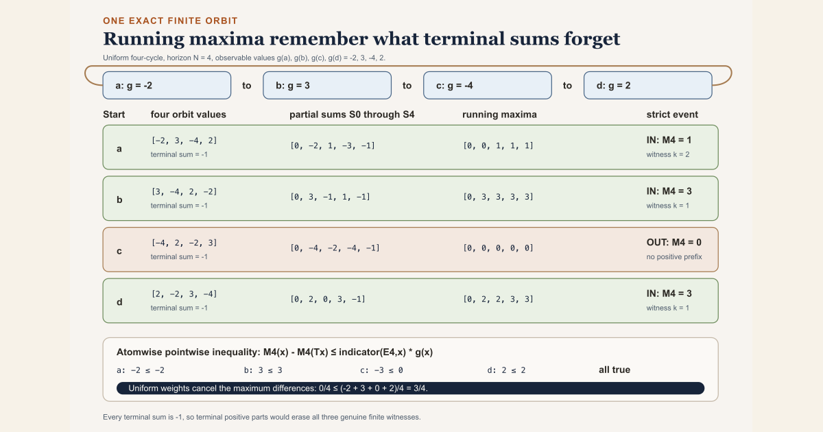
Begin with four equally weighted states
Take the finite state space
\[ \Omega=\{a,b,c,d\} \]with the uniform probability measure, so every state has mass \(1/4\). Let the transformation cycle through the states:
\[ a\longmapsto b\longmapsto c\longmapsto d\longmapsto a. \]This map preserves the uniform measure because it only permutes four equal atoms. Define the real observable
\[ g(a)=-2,\qquad g(b)=3,\qquad g(c)=-4,\qquad g(d)=2. \]Fix horizon \(N=4\). For each starting state \(x\), the finite Birkhoff sum \(S_k g(x)\) adds the first \(k\) values seen from \(x\). The empty sum \(S_0g(x)\) is zero. The complete ledger is:
| start \(x\) | orbit values through four steps | \(S_0,S_1,S_2,S_3,S_4\) | running maxima | final \(M_4g(x)\) | \(0\lt M_4g(x)\)? |
|---|---|---|---|---|---|
| \(a\) | \(-2,3,-4,2\) | \(0,-2,1,-3,-1\) | \(0,0,1,1,1\) | \(1\) | yes |
| \(b\) | \(3,-4,2,-2\) | \(0,3,-1,1,-1\) | \(0,3,3,3,3\) | \(3\) | yes |
| \(c\) | \(-4,2,-2,3\) | \(0,-4,-2,-4,-1\) | \(0,0,0,0,0\) | \(0\) | no |
| \(d\) | \(2,-2,3,-4\) | \(0,2,0,3,-1\) | \(0,2,2,3,3\) | \(3\) | yes |
All four terminal sums are \(-1\). Looking only at time four would therefore miss every positive prefix. The running maximum remembers them, and the strict finite Hopf event is
\[ E_4(g)=\{a,b,d\}. \]State \(a\) is the instructive atom. Its first observable value is negative, yet its two-step sum is
\[ -2+3=1\gt0. \]The theorem does not say \(g(x)\) is pointwise nonnegative on the event.
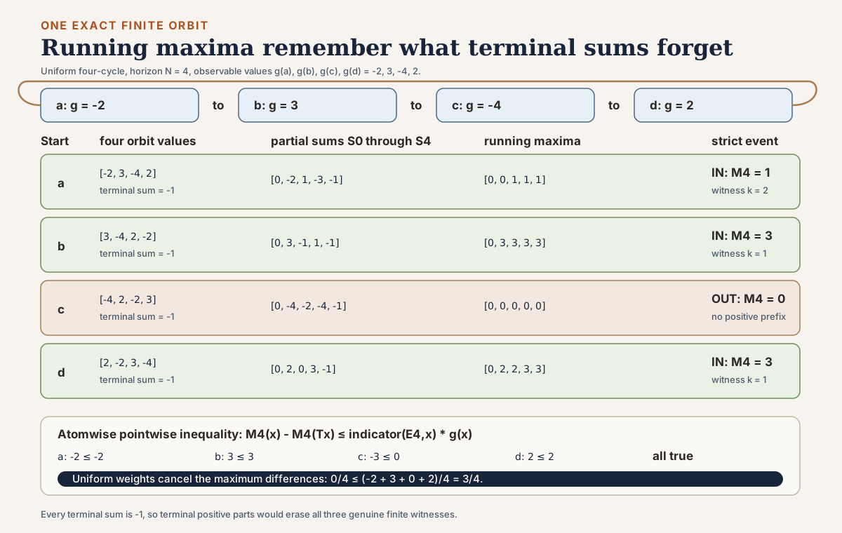
See the pointwise inequality atom by atom
The proof’s finite pointwise statement is
\[ M_4g(x)-M_4g(Tx) \le \mathbf 1_{E_4(g)}(x)g(x). \]For this cycle, no abstraction is needed:
| atom \(x\) | \(M_4g(x)\) | \(M_4g(Tx)\) | difference | \(\mathbf 1_{E_4(g)}(x)g(x)\) | check |
|---|---|---|---|---|---|
| \(a\) | \(1\) | \(3\) | \(-2\) | \(-2\) | equality |
| \(b\) | \(3\) | \(0\) | \(3\) | \(3\) | equality |
| \(c\) | \(0\) | \(3\) | \(-3\) | \(0\) | \(-3\le0\) |
| \(d\) | \(3\) | \(1\) | \(2\) | \(2\) | equality |
The uniform integral is just the average of four atom values. The maximum differences cancel around the cycle:
\[ \frac{-2+3-3+2}{4}=0. \]The indicator side is
\[ \frac{-2+3+0+2}{4} =\int_{E_4(g)}g\,d\mu =\frac34. \]Thus the finite Hopf conclusion is visible before any general integration machinery:
\[ 0\le\int_{E_4(g)}g\,d\mu. \]Turn the same orbit into an average-threshold event
For positive \(k\), divide each partial sum by \(k\). The four average rows are:
| start | \(A_1,A_2,A_3,A_4\) | some average strictly above \(1\)? |
|---|---|---|
| \(a\) | \(-2,\frac12,-1,-\frac14\) | no |
| \(b\) | \(3,-\frac12,\frac13,-\frac14\) | yes |
| \(c\) | \(-4,-1,-\frac43,-\frac14\) | no |
| \(d\) | \(2,0,1,-\frac14\) | yes |
At strict threshold \(a=1\),
\[ E_{4,1}(g)=\{b,d\}, \qquad \mu(E_{4,1}(g))=\frac12. \]The third average from \(d\) equals one and therefore does not qualify, but its first average is two, so \(d\) still has a strict witness. The exact integral chain is
\[ 1\cdot\frac12 \le \int_{\{b,d\}}g\,d\mu =\frac{3+2}{4} =\frac54 \le \int_\Omega\max(g,0)\,d\mu =\frac54. \]Dividing by the positive threshold one gives the finite weak estimate \(\frac12\le\frac54\).
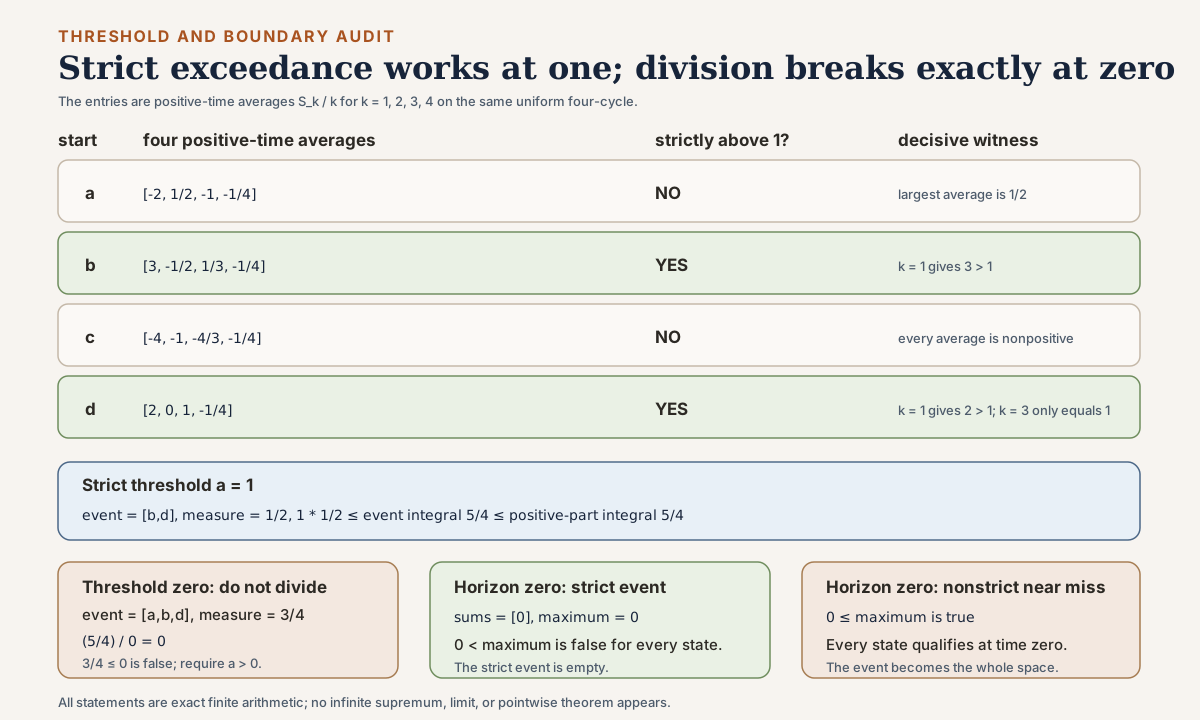
Two boundaries fix the theorem statements
First set the threshold to zero. The strict positive-average event is \(\{a,b,d\}\), with mass \(3/4\). The undivided theorem still gives a valid statement whose left side is zero. But a putative weak theorem without \(0\lt a\) would read
\[ \frac34 \le \frac{\int g^+\,d\mu}{0} =0, \]which is false under Lean’s total division. Threshold positivity is needed exactly when division occurs, not in the preceding multiplication estimate.
Now set the horizon to zero. Every partial-sum list is just \([0]\), and every maximum is zero. Therefore
\[ E_0(g)=\varnothing. \]If the event were defined nonstrictly by \(0\le M_0g\), all four states would qualify at time zero. In fact, because every finite maximum includes the zero sum, the nonstrict event is the whole space at every horizon. This is why the formal definition uses strict positivity.
Suppose a real observable is read along an orbit. At each finite time one can add everything seen so far, then ask whether any of those running totals is positive. That question remembers the whole finite prefix, not only its last sum. It is exactly the kind of pathwise selection that can look difficult to integrate: each starting point may choose a different winning time.
The finite maximal ergodic argument avoids integrating the chosen time. It packages all choices into one maximum. Strict positivity ensures that a maximizer occurs at a positive time. The first summand can then be peeled from that winning sum, leaving a partial sum along the shifted orbit. When the transformation preserves the measure, the original and shifted maxima have the same integral. Their difference cancels, and what remains is a nonnegative integral of the observable over the strict event.
Random-matrix-theory milestone 23 (RMT-23) formalizes this finite mechanism in Lean. The compact concept page is finite maximal ergodic inequality . The declaration-complete implementation account is The Finite Hopf Maximal Ergodic Lemma in Lean. The immediate conceptual predecessor is Birkhoff Convergence Events Before the Pointwise Ergodic Theorem.
Choose a route up
| Route | Begin | Destination |
|---|---|---|
| Orbit route | Start with finite orbit sums | Reconstruct the sum convention |
| Geometry route | Put time zero inside the maximum | Understand strict versus nonstrict selection |
| Measure route | Measurability and integrability are different gates | Track exact analytic premises |
| Pointwise route | Peel a positive maximizing index | Prove the indicator inequality |
| Integral route | Preservation performs the cancellation | Derive the finite Hopf lemma |
| Threshold route | Center by a threshold, not by an expectation | Identify finite average exceedances |
| Weak route | Divide only after proving positivity | Obtain the horizon-uniform estimate |
| History route | Four sources, four different scopes | Preserve attribution and notation |
| Lean route | The complete twenty-five-declaration ledger | Audit every public name |
| Boundary route | Eleven probes guard the theorem boundary | Test zero, infinite measure, and failed preservation |
| Summit route | What remains after the finite estimate | Locate the finite-to-infinite gap |
Learning objectives
By the summit, a reader should be able to:
- state the exact zero-based convention for a finite Birkhoff sum;
- distinguish a running maximum from the positive part of a terminal sum;
- explain why including time zero makes the maximum nonnegative;
- explain why a nonstrict event would be the entire state space;
- rewrite strict-event membership as a positive-time witness;
- derive the horizon-zero and horizon-one boundaries;
- prove that finite maxima increase with the horizon;
- derive ordinary measurability of a finite maximum;
- derive integrability of a finite maximum under preservation;
- distinguish ordinary measurability from almost-everywhere strong measurability;
- choose a maximizing index without making it a measurable function;
- prove that a positive maximizing index cannot be zero;
- peel the first observable value from a successor Birkhoff sum;
- compare the remainder with the shifted running maximum;
- handle the complement of the strict event without a maximizing witness;
- combine the two pointwise branches with an indicator;
- explain precisely where measure preservation enters;
- derive the cancellation of the two maximal-function integrals;
- state the finite Hopf-style integral inequality;
- explain why no finite-measure or probability premise is needed there;
- explain why neither injectivity nor invertibility is needed;
- encode an average-threshold event using \(g-a\);
- prove the centered-sum identity and membership equivalence;
- locate the exact reason a finite-measure premise appears for centering;
- derive the threshold integral lower bound for every real \(a\);
- replace \(g\) by its positive part on the right side;
- identify why \(a\gt0\) is needed only for division;
- distinguish a finite-horizon estimate from an infinite maximal theorem;
- describe the contributions and limits of the four historical sources;
- map all twenty-five public declarations to their proof layers;
- interpret all eleven compiled boundary probes; and
- state the exact remaining work toward a pointwise ergodic theorem.
Common setup and notation
Let:
- \(\Omega\) be a type equipped with a measurable space;
- \(\mu\) be a measure on \(\Omega\);
- \(T:\Omega\to\Omega\) be a discrete-time transformation;
- \(T^j\) be the \(j\)-fold iterate of \(T\);
- \(g:\Omega\to\mathbb R\) be a real observable;
- \(N\in\mathbb N\) be a fixed finite horizon;
- \(k\in\mathbb N\) be a candidate time; and
- \(\omega\in\Omega\) be a starting point.
Write
\[ S_kg(\omega) {} = \sum_{\substack{j\in\mathbb N\\j\lt k}} g\bigl(T^j\omega\bigr) \]for the finite Birkhoff sum. Write
\[ M_Ng(\omega)=\max_{0\le k\le N}S_kg(\omega) \]for the running maximum through time \(N\), and
\[ E_N(g)=\{\omega:0\lt M_Ng(\omega)\} \]for its strict positivity event.
When a threshold \(a\in\mathbb R\) is present, write
\[ A_kg(\omega)=\frac{S_kg(\omega)}{k} \qquad(k\ge1) \]and
\[ E_{N,a}(g) {} = \left\{\omega: \exists k,\ 1\le k\le N,\ a\lt A_kg(\omega) \right\}. \]The restriction \(k\ge1\) matters because the average at time zero is totalized in Lean but division is only order-reflecting at a positive denominator.
Start with finite orbit sums
Mathlib’s
finite Birkhoff sum uses
Finset.range k. That range contains the natural numbers strictly
below \(k\). Consequently,
Two successor identities are useful, and they peel opposite ends:
\[ \begin{aligned} S_{k+1}g(\omega) &=S_kg(\omega)+g(T^k\omega),\\ S_{k+1}g(\omega) &=g(\omega)+S_kg(T\omega). \end{aligned} \]The maximal proof uses the second identity. It removes the first orbit value and leaves the same observable along the orbit starting at \(T\omega\).
The finite maximum is encoded with a nonempty finite supremum:
def finiteBirkhoffSumMax (T : Ω → Ω) (g : Ω → ℝ) (N : ℕ) : Ω → ℝ :=
  fun ω ↦
    (Finset.range (N + 1)).sup' Finset.nonempty_range_add_one
      (fun k ↦ birkhoffSum T g k ω)
The range \(N+1\) contains exactly \(0,\ldots,N\). The proof object
Finset.nonempty_range_add_one certifies that sup’
really has an element to maximize. This avoids inventing a default maximum
outside the mathematical index set.
Every candidate sum lies below the maximum:
\[ k\le N\quad\Longrightarrow\quad S_kg(\omega)\le M_Ng(\omega). \]If \(M\le N\), every index available at horizon \(M\) remains available at horizon \(N\). Hence
\[ M_Mg(\omega)\le M_Ng(\omega). \]This is monotonicity in the horizon, not monotonicity of the individual partial sums. The sequence \(S_kg(\omega)\) may rise and fall.
Put time zero inside the maximum
Since \(S_0g(\omega)=0\) and zero is one of the maximized values,
\[ 0\le M_Ng(\omega) \]for every map, observable, horizon, and point. No measurable structure is needed.
At horizon zero there is only one candidate:
\[ M_0g(\omega)=S_0g(\omega)=0. \]These two small facts determine the event convention. If one defined
\[ F_N(g)=\{\omega:0\le M_Ng(\omega)\}, \]then \(F_N(g)=\Omega\) for every \(g\). It would remember nothing about the positive-time orbit. The strict event
\[ E_N(g)=\{\omega:0\lt M_Ng(\omega)\} \]removes that degeneracy.
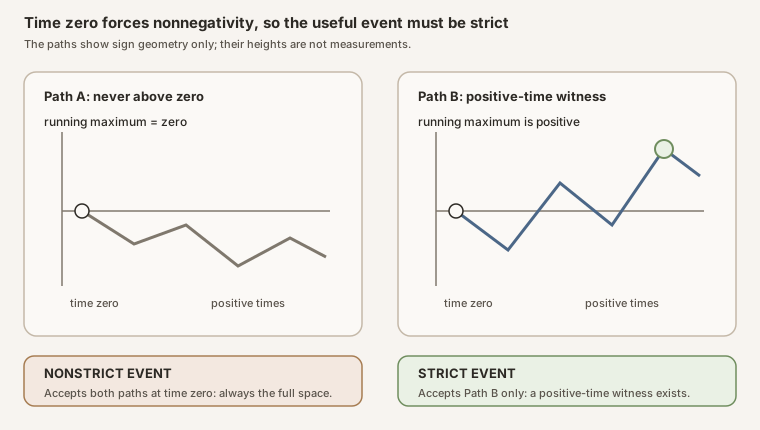
The exact membership theorem is
\[ \omega\in E_N(g) \quad\Longleftrightarrow\quad \exists k,\ 1\le k\le N\ \text{ and }\ 0\lt S_kg(\omega). \]For the forward direction, strict positivity of a finite supremum supplies an index with positive value. That index cannot be zero because \(S_0=0\). For the reverse direction, any positive candidate is bounded above by the maximum, so the maximum is positive.
Two boundaries follow:
\[ E_0(g)=\varnothing, \qquad \omega\in E_1(g)\Longleftrightarrow 0\lt g(\omega). \]The event also increases with its horizon. A positive witness available by time \(M\) remains available by time \(N\) whenever \(M\le N\).
Measurability and integrability are different gates
The finite maximum has both an ordinary-measurability route and an integrability route. They should not be collapsed.
Ordinary measurability
Assume \(T\) and \(g\) are measurable. Every finite iterate \(T^j\) is measurable, every composition \(g\circ T^j\) is measurable, and every finite Birkhoff sum is measurable. A finite supremum of measurable real functions is measurable through Mathlib’s finite lattice API. Therefore
\[ \omega\longmapsto M_Ng(\omega) \]is measurable, and the strict superlevel comparison
\[ E_N(g)=\{\omega:0\lt M_Ng(\omega)\} \]is a measurable set.
This route mentions no measure. It cannot require preservation, probability, integrability, or ergodicity.
Integrability
Assume instead that \(T\) preserves \(\mu\) and \(g\) is integrable with respect to \(\mu\). Preservation propagates integrability along every finite iterate, so each \(g\circ T^j\) is integrable. Finite sums remain integrable. The maximum of two integrable real functions is integrable, and finite induction closes the whole maximum.
Thus
\[ M_Ng\in L^1(\mu). \]This theorem does not require \(\mu(\Omega)\lt\infty\). It does not require a probability measure. The integrability of \(g\) controls the finitely many orbit terms, while preservation keeps their integrals from changing under composition.
An integrable function in Mathlib is almost-everywhere strongly measurable.
That does not assert ordinary measurability of the exact representative
supplied by the caller. RMT-23 therefore derives
NullMeasurableSet (finiteHopfEvent T g N) μ directly from the
almost-everywhere measurability of the integrable maximum. This is exactly the
set interface needed by indicator integrability and set integration. The
almost everywhere
entry explains the
representative distinction.
Peel a positive maximizing index
Fix \(\omega\in E_N(g)\). Because the index set is finite and nonempty, some \(k\le N\) attains the maximum:
\[ M_Ng(\omega)=S_kg(\omega). \]The maximum is positive, so \(S_kg(\omega)\gt0\). Time zero has sum zero, hence \(k\ne0\). There is a natural number \(j\) with \(k=j+1\).
Now apply the first-summand successor identity:
\[ \begin{aligned} M_Ng(\omega) &=S_{j+1}g(\omega)\\ &=g(\omega)+S_jg(T\omega)\\ &\le g(\omega)+M_Ng(T\omega). \end{aligned} \]The last step is valid because \(j\le N\). In fact \(j\lt N\), but the weaker bound is enough to place \(S_jg(T\omega)\) among the terms maximized by \(M_Ng(T\omega)\).
Rearrange:
\[ M_Ng(\omega)-M_Ng(T\omega)\le g(\omega). \]This is the on-event branch.
Now suppose \(\omega\notin E_N(g)\). The maximum is nonnegative everywhere, yet it is not positive here. Therefore
\[ M_Ng(\omega)=0. \]The shifted maximum remains nonnegative, so
\[ M_Ng(\omega)-M_Ng(T\omega) {} = -M_Ng(T\omega) \le0. \]This is the off-event branch. It needs no selected maximizer.
Combining them gives the global pointwise inequality
\[ M_Ng(\omega)-M_Ng(T\omega) \le \mathbf 1_{E_N(g)}(\omega)\,g(\omega). \]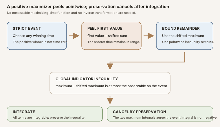
This proof architecture is close to Garsia’s concise 1965 presentation, but the Lean theorem fixes its exact finite range and strict event explicitly. The running maximum is not the positive part of the terminal sum. A terminal sum can be negative even though an earlier partial sum was positive.
Preservation performs the cancellation
The pointwise inequality becomes useful only after all terms are known to be integrable. Let
\[ M(\omega)=M_Ng(\omega), \qquad E=E_N(g). \]The integrability theorem supplies \(M\in L^1(\mu)\). Measure preservation also gives \(M\circ T\in L^1(\mu)\). The null-measurable event theorem makes \(\mathbf1_Eg\) integrable.
Monotonicity of the integral applied to the pointwise inequality yields
\[ \int_\Omega \bigl(M(\omega)-M(T\omega)\bigr)\,d\mu(\omega) \le \int_\Omega \mathbf1_E(\omega)g(\omega)\,d\mu(\omega). \]The private helper integral_comp_of_measurePreserving proves
Its proof uses Mathlib’s
integral_map
and the equality of the pushforward measure with \(\mu\). Therefore the entire
left side is zero:
The indicator integral is the set integral, so
\[ \boxed{ 0\le\int_{E_N(g)}g\,d\mu. } \]This is integral_finiteHopfEvent_nonneg.
Why the assumptions are genuinely weak
The theorem needs:
- a measurable space on \(\Omega\), so measure theory is meaningful;
- a measure \(\mu\);
MeasurePreserving T μ μ; andIntegrable g μ.
It does not need:
- \(\mu(\Omega)\lt\infty\);
- probability normalization;
- a sigma-finite measure;
- ergodicity;
- injectivity;
- surjectivity;
- invertibility; or
- an ordinarily measurable raw representative for \(g\).
The bundled MeasurePreserving premise includes measurability of
\(T\). The proof also uses its pushforward equality. It never asks for a
preimage point or an inverse transformation.
The infinite counting-measure probe is especially instructive. On \(\mathbb N\) with counting measure, take the identity transformation and an integrable point mass. The total measure is infinite, but the theorem still applies. Finite measure appears only later when a nonzero constant threshold must itself be integrable.
Center by a threshold, not by an expectation
Fix \(a\in\mathbb R\) and define
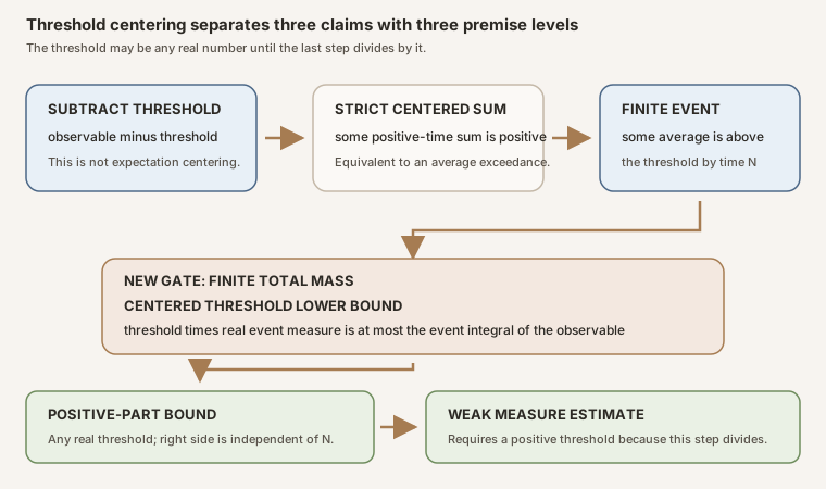
\[ h(\omega)=g(\omega)-a. \]This is threshold centering. It does not say that \(h\) has integral zero. Unless \(a\) has been chosen from a normalized expectation and the needed integral identity has been proved, “mean centered” would overstate the construction.
Finite sums respect subtraction:
\[ \begin{aligned} S_kh(\omega) &=S_k(g-a)(\omega)\\ &=S_kg(\omega)-S_k(a)(\omega)\\ &=S_kg(\omega)-ka. \end{aligned} \]For \(k\ge1\), multiplication or division by \(k\gt0\) preserves strict order:
\[ 0\lt S_kh(\omega) \quad\Longleftrightarrow\quad a\lt\frac{S_kg(\omega)}{k}. \]Therefore
\[ E_N(h)=E_{N,a}(g) {} = \left\{\omega: \exists k,\ 1\le k\le N,\ a\lt A_kg(\omega) \right\}. \]RMT-23 names this set
finiteBirkhoffAverageExceedanceSet T g N a. It is a union over a
finite range of positive horizons, encoded through one already developed
strict maximal event.
The event increases with \(N\). Ordinary measurability follows from
measurability of \(T\) and \(g\). Its null-measurable integrability route adds
[IsFiniteMeasure μ] because the constant function \(\omega\mapsto
a\) must be integrable before \(g-a\) can be fed to the finite Hopf lemma.
The threshold integral inequality
Assume now that \(\mu\) is finite, \(T\) preserves \(\mu\), and \(g\) is integrable. Apply the core lemma to \(h=g-a\) and \(E=E_{N,a}(g)\):
\[ 0\le\int_E(g-a)\,d\mu. \]Set-integral subtraction and integration of a constant over a set give
\[ \begin{aligned} 0 &\le \int_Eg\,d\mu-\int_Ea\,d\mu\\ &=\int_Eg\,d\mu-a\,\mu_{\mathbb R}(E). \end{aligned} \]Thus
\[ \boxed{ a\,\mu_{\mathbb R}\bigl(E_{N,a}(g)\bigr) \le \int_{E_{N,a}(g)}g\,d\mu. } \]The notation \(\mu_{\mathbb R}\) is Mathlib’s finite real-valued measure projection. The displayed inequality is valid for every \(a\in\mathbb R\), including zero and negative thresholds.
The sign must remain explicit: the argument has not divided by \(a\), so it does not require a sign assumption on \(a\). For negative \(a\), the left side is nonpositive because the event measure is nonnegative. The result remains correct even when it is not a useful upper bound on the event’s size.
Remove the event from the right side
Define the positive part
\[ g^+(\omega)=\max(g(\omega),0). \]Pointwise, \(g\le g^+\). Therefore
\[ \int_Eg\,d\mu\le\int_Eg^+\,d\mu. \]Since \(g^+\ge0\), restricting its integral to a set cannot exceed its integral over the whole space:
\[ \int_Eg^+\,d\mu\le\int_\Omega g^+\,d\mu. \]Combining these inequalities gives the horizon-uniform bound
\[ \boxed{ a\,\mu_{\mathbb R}\bigl(E_{N,a}(g)\bigr) \le \int_\Omega g^+\,d\mu. } \]The right side depends on \(g\) and \(\mu\), but not on \(N\). This uniformity is what makes the finite statement useful in a future monotone limiting argument.
The notation \(g^+\) here really is a pointwise positive part. This should not be confused with Garsia’s historical notation \(S_n^+\), which denotes a running maximum of several partial sums in the cited proof.
Divide only after proving positivity
If \(a\gt0\), division preserves the inequality:
\[ \boxed{ \mu_{\mathbb R}\bigl(E_{N,a}(g)\bigr) \le \frac{\int_\Omega g^+\,d\mu}{a}. } \]This is a weak finite maximal estimate. The phrase weak refers to control of the measure of a threshold event rather than pointwise control of every average.
The proof signature makes the timing exact:
finiteBirkhoffAverageExceedanceSet_integral_lower_boundaccepts any real \(a\);finiteBirkhoffAverageExceedanceSet_posPart_boundalso accepts any real \(a\); andmeasureReal_finiteBirkhoffAverageExceedanceSet_lealone takesha : 0 < a.
At \(a=0\), the division theorem would be meaningless. At \(a\lt0\), dividing would reverse order. The earlier integral inequalities remain valid because they do neither operation.
Seven bridges from the orbit ledger to Lean
The first four bridges build the finite Hopf inequality. The last three turn it into a threshold-event estimate. Each Lean expression names an exact project declaration; the copyable module probe and full project command follow the bridges.
Bridge 1: maximize every partial sum, including time zero
finiteBirkhoffSumMax T g N ωfiniteBirkhoffSumMaxis a function of the startω.Finset.range (N + 1)supplies exactly the indices \(0,\ldots,N\).sup’takes a maximum over a proved nonempty finite set.- The candidate at
k = 0isbirkhoffSum … 0 = 0.
Bridge 2: strict event membership produces a positive-time witness
mem_finiteHopfEvent_ifffiniteHopfEvent T g Nis the set \(E_N(g)\).- The witness has
1 ≤ k, so it cannot be the forced zero-time candidate. k ≤ Nincludes the terminal horizon.- The rightmost comparison remains strict, matching the worked event \(\{a,b,d\}\).
Bridge 3: combine the selected and unselected atoms
finiteBirkhoffSumMax_sub_comp_le_indicator (T := T) (g := g) N ω(T := T)and(g := g)fill implicit arguments explicitly for a readable call.Set.indicatorreturnsg ωon the event and zero outside it.- The proof peels a positive maximizing successor index only on the event.
- Off the event, nonnegativity and failure of strict positivity force the current maximum to equal zero.
Bridge 4: preservation cancels the shifted maximum
integral_finiteHopfEvent_nonneg hT hg NhT : MeasurePreserving T μ μsupplies measurability and the pushforward equality, not ergodicity.hg : Integrable g μmakes every finite sum and finite maximum integrable.- Preservation proves \(\int M_Ng\circ T\,d\mu=\int M_Ng\,d\mu\).
- No finite-total-mass, probability, injectivity, or invertibility premise is present.
Bridge 5: threshold centering is exactly average exceedance
mem_finiteBirkhoffAverageExceedanceSet_ifffiniteBirkhoffAverageExceedanceSet T g N ais defined as the finite Hopf event offun ω ↦ g ω - a.birkhoffAverage ℝ T g k ωis the real average at timek.- Positivity of
klicenses the strict order-preserving division. - The threshold is pointwise centering, not expectation centering.
Bridge 6: remove the event from the right side
finiteBirkhoffAverageExceedanceSet_posPart_bound hT hg N a[IsFiniteMeasure μ]makes the constant threshold integrable.μ.realis Mathlib’s real-valued view of a finite measure.max (g ω) 0is the pointwise positive part \(g^+\).amay be negative, zero, or positive because this theorem does not divide by it.
Bridge 7: divide only with a positive threshold
measureReal_finiteBirkhoffAverageExceedanceSet_le hT hg N haha : 0 < ais the proof consumed byle_div_iff₀.- The event and positive-part integral are the same objects as in bridge 6.
- The right side does not depend on
N, but the event is still finite-horizon. - The zero-threshold worksheet shows why dropping
hawould make the divided conclusion false.
Type-check the exact project interface
For a full project check, place this probe in a project scratch file after installing the repository’s pinned dependencies:
import NonlinearDynamics.Random.RandomCocycles.FiniteHopfMaximal

open NonlinearDynamics.Random.RandomCocycles

#check finiteBirkhoffSumMax
#check finiteBirkhoffSumMax_nonneg
#check mem_finiteHopfEvent_iff
#check finiteBirkhoffSumMax_sub_comp_le_indicator
#check integral_finiteHopfEvent_nonneg
#check mem_finiteBirkhoffAverageExceedanceSet_iff
#check finiteBirkhoffAverageExceedanceSet_posPart_bound
#check measureReal_finiteBirkhoffAverageExceedanceSet_le
From the repository root, type:
cd formalization
lake env lean NonlinearDynamics/Random/RandomCocycles/FiniteHopfMaximal.lean
This is a full project check. It may compile substantial dependencies and therefore may require substantial disk space and memory. It checks the authoritative 509-line module.
cd formalization
lake env lean -DwarningAsError=true NonlinearDynamics/Random/RandomCocycles/FiniteHopfMaximal.lean
Resource note: this exact file uses the repository's
pinned Lean and Mathlib dependencies. Initial project setup can require
substantial disk space and build time. For a lightweight first step on
macOS or Linux, use the page's standalone Lean-core or Std
tutorial.
Run the entire four-cycle ledger with Std
The following file imports only Lean’s Std library. It defines its own
four-cycle, finite sums, running maxima, rational averages, indicators, and
uniform atom integrals. It does not import Mathlib or the project. Save the
block byte for byte as
/tmp/FiniteHopfMaximalDeepDiveTutorial.lean:
import Std

namespace FiniteHopfMaximalDeepDiveTutorial

inductive OrbitState where
  | a
  | b
  | c
  | d
  deriving Repr, DecidableEq

def states : List OrbitState :=
  [.a, .b, .c, .d]

def stateName : OrbitState → String
  | .a => "a"
  | .b => "b"
  | .c => "c"
  | .d => "d"

def step : OrbitState → OrbitState
  | .a => .b
  | .b => .c
  | .c => .d
  | .d => .a

def observable : OrbitState → Int
  | .a => -2
  | .b => 3
  | .c => -4
  | .d => 2

def iterate : Nat → OrbitState → OrbitState
  | 0, x => x
  | n + 1, x => iterate n (step x)

def orbitSum : Nat → OrbitState → Int
  | 0, _ => 0
  | n + 1, x => orbitSum n x + observable (iterate n x)

def orbitValues (horizon : Nat) (x : OrbitState) : List Int :=
  (List.range horizon).map fun j => observable (iterate j x)

def partialSums (horizon : Nat) (x : OrbitState) : List Int :=
  (List.range (horizon + 1)).map fun k => orbitSum k x

def runningMaximaFrom : Int → List Int → List Int
  | _, [] => []
  | current, value :: rest =>
      let next := max current value
      next :: runningMaximaFrom next rest

def runningMaxima (horizon : Nat) (x : OrbitState) : List Int :=
  runningMaximaFrom 0 (partialSums horizon x)

def finiteMax (horizon : Nat) (x : OrbitState) : Int :=
  (partialSums horizon x).foldl max 0

def inStrictEvent (horizon : Nat) (x : OrbitState) : Bool :=
  decide (0 < finiteMax horizon x)

def inNonstrictEvent (horizon : Nat) (x : OrbitState) : Bool :=
  decide (0 ≤ finiteMax horizon x)

def average (k : Nat) (x : OrbitState) : Rat :=
  (orbitSum k x : Rat) / (k : Rat)

def positiveTimeAverages (horizon : Nat) (x : OrbitState) : List Rat :=
  (List.range horizon).map fun j => average (j + 1) x

def exceedsAverage
    (horizon : Nat) (threshold : Rat) (x : OrbitState) : Bool :=
  (List.range horizon).any fun j =>
    decide (threshold < average (j + 1) x)

def selectedStates (horizon : Nat) : List OrbitState :=
  states.filter fun x => inStrictEvent horizon x

def thresholdStates
    (horizon : Nat) (threshold : Rat) : List OrbitState :=
  states.filter fun x => exceedsAverage horizon threshold x

def indicatorContribution (horizon : Nat) (x : OrbitState) : Int :=
  if inStrictEvent horizon x then observable x else 0

def sumObservable (selected : List OrbitState) : Int :=
  selected.foldl (fun total x => total + observable x) 0

def quarterIntegral (numerator : Int) : Rat :=
  (numerator : Rat) / 4

def positivePartSum : Int :=
  states.foldl (fun total x => total + max (observable x) 0) 0

structure OrbitRow where
  start : String
  values : List Int
  sums : List Int
  maxima : List Int
  strictPositive : Bool
  averages : List Rat
  averageAboveOne : Bool
  deriving Repr, DecidableEq

def orbitRow (x : OrbitState) : OrbitRow :=
  { start := stateName x
    values := orbitValues 4 x
    sums := partialSums 4 x
    maxima := runningMaxima 4 x
    strictPositive := inStrictEvent 4 x
    averages := positiveTimeAverages 4 x
    averageAboveOne := exceedsAverage 4 1 x }

structure PointwiseRow where
  start : String
  maximumHere : Int
  maximumAfterStep : Int
  difference : Int
  indicatorTimesObservable : Int
  inequalityHolds : Bool
  deriving Repr, DecidableEq

def pointwiseRow (x : OrbitState) : PointwiseRow :=
  let here := finiteMax 4 x
  let shifted := finiteMax 4 (step x)
  let contribution := indicatorContribution 4 x
  { start := stateName x
    maximumHere := here
    maximumAfterStep := shifted
    difference := here - shifted
    indicatorTimesObservable := contribution
    inequalityHolds := decide (here - shifted ≤ contribution) }

structure IntegralLedger where
  strictEvent : List String
  maxDifferenceNumerator : Int
  indicatorNumerator : Int
  eventIntegral : Rat
  thresholdOneEvent : List String
  thresholdOneMeasure : Rat
  thresholdOneLeftSide : Rat
  thresholdOneEventIntegral : Rat
  positivePartIntegral : Rat
  weakBoundAtOneHolds : Bool
  zeroThresholdEvent : List String
  zeroThresholdMeasure : Rat
  dividedRightAtZero : Rat
  weakBoundAtZeroWouldHold : Bool
  zeroHorizonStrictEvent : List String
  zeroHorizonNonstrictEvent : List String
  deriving Repr, DecidableEq

def integralLedger : IntegralLedger :=
  let strict := selectedStates 4
  let pointwise := states.map pointwiseRow
  let differenceTotal :=
    pointwise.foldl (fun total row => total + row.difference) 0
  let indicatorTotal :=
    pointwise.foldl
      (fun total row => total + row.indicatorTimesObservable) 0
  let thresholdOne := thresholdStates 4 1
  let thresholdZero := thresholdStates 4 0
  let positiveIntegral := quarterIntegral positivePartSum
  { strictEvent := strict.map stateName
    maxDifferenceNumerator := differenceTotal
    indicatorNumerator := indicatorTotal
    eventIntegral := quarterIntegral indicatorTotal
    thresholdOneEvent := thresholdOne.map stateName
    thresholdOneMeasure := (thresholdOne.length : Rat) / 4
    thresholdOneLeftSide := 1 * ((thresholdOne.length : Rat) / 4)
    thresholdOneEventIntegral :=
      quarterIntegral (sumObservable thresholdOne)
    positivePartIntegral := positiveIntegral
    weakBoundAtOneHolds :=
      decide ((thresholdOne.length : Rat) / 4 ≤ positiveIntegral / 1)
    zeroThresholdEvent := thresholdZero.map stateName
    zeroThresholdMeasure := (thresholdZero.length : Rat) / 4
    dividedRightAtZero := positiveIntegral / 0
    weakBoundAtZeroWouldHold :=
      decide ((thresholdZero.length : Rat) / 4 ≤ positiveIntegral / 0)
    zeroHorizonStrictEvent :=
      (states.filter fun x => inStrictEvent 0 x).map stateName
    zeroHorizonNonstrictEvent :=
      (states.filter fun x => inNonstrictEvent 0 x).map stateName }

#eval states.map orbitRow
#eval states.map pointwiseRow
#eval integralLedger

example : partialSums 4 .a = [0, -2, 1, -3, -1] := by
  native_decide
example : partialSums 4 .b = [0, 3, -1, 1, -1] := by
  native_decide
example : partialSums 4 .c = [0, -4, -2, -4, -1] := by
  native_decide
example : partialSums 4 .d = [0, 2, 0, 3, -1] := by
  native_decide

example : runningMaxima 4 .a = [0, 0, 1, 1, 1] := by
  native_decide
example : runningMaxima 4 .b = [0, 3, 3, 3, 3] := by
  native_decide
example : runningMaxima 4 .c = [0, 0, 0, 0, 0] := by
  native_decide
example : runningMaxima 4 .d = [0, 2, 2, 3, 3] := by
  native_decide

example : selectedStates 4 = [.a, .b, .d] := by
  native_decide
example : thresholdStates 4 1 = [.b, .d] := by
  native_decide
example : thresholdStates 4 0 = [.a, .b, .d] := by
  native_decide

example : (states.map pointwiseRow).map PointwiseRow.difference =
    [-2, 3, -3, 2] := by native_decide
example : (states.map pointwiseRow).map
    PointwiseRow.indicatorTimesObservable = [-2, 3, 0, 2] := by
  native_decide
example : (states.map pointwiseRow).all PointwiseRow.inequalityHolds = true := by
  native_decide

example : integralLedger.eventIntegral = (3 : Rat) / 4 := by
  native_decide
example : integralLedger.thresholdOneMeasure = (1 : Rat) / 2 := by
  native_decide
example : integralLedger.thresholdOneEventIntegral = (5 : Rat) / 4 := by
  native_decide
example : integralLedger.positivePartIntegral = (5 : Rat) / 4 := by
  native_decide
example : integralLedger.weakBoundAtOneHolds = true := by
  native_decide
example : integralLedger.dividedRightAtZero = 0 := by
  native_decide
example : integralLedger.weakBoundAtZeroWouldHold = false := by
  native_decide
example : integralLedger.zeroHorizonStrictEvent = [] := by
  native_decide
example : integralLedger.zeroHorizonNonstrictEvent =
    ["a", "b", "c", "d"] := by
  native_decide

end FiniteHopfMaximalDeepDiveTutorial
The key syntax is ordinary and finite:
inductive OrbitStatecreates exactly four named states;iterateadvances the cycle without importing Mathlib’s iterate API;List.range (horizon + 1)includes the zero-time sum;foldl max 0accumulates a running finite maximum from the forced zero;Ratkeeps all averages and uniform atom integrals exact;decidecomputes a finite comparison; and- every
native_decideexample supplies a kernel-checked proof of the displayed ledger.
With the pinned compiler installed, a human types:
source "$HOME/.elan/env"
elan run leanprover/lean4:v4.32.0 lean \
  /tmp/FiniteHopfMaximalDeepDiveTutorial.lean
This is a standalone tutorial suitable for a normal macOS or Linux
host. It imports only Std, enumerates four states, and does not compile
Mathlib or this project. Successful execution prints exactly:
[{ start := "a",
   values := [-2, 3, -4, 2],
   sums := [0, -2, 1, -3, -1],
   maxima := [0, 0, 1, 1, 1],
   strictPositive := true,
   averages := [-2, (1 : Rat)/2, -1, (-1 : Rat)/4],
   averageAboveOne := false },
 { start := "b",
   values := [3, -4, 2, -2],
   sums := [0, 3, -1, 1, -1],
   maxima := [0, 3, 3, 3, 3],
   strictPositive := true,
   averages := [3, (-1 : Rat)/2, (1 : Rat)/3, (-1 : Rat)/4],
   averageAboveOne := true },
 { start := "c",
   values := [-4, 2, -2, 3],
   sums := [0, -4, -2, -4, -1],
   maxima := [0, 0, 0, 0, 0],
   strictPositive := false,
   averages := [-4, -1, (-4 : Rat)/3, (-1 : Rat)/4],
   averageAboveOne := false },
 { start := "d",
   values := [2, -2, 3, -4],
   sums := [0, 2, 0, 3, -1],
   maxima := [0, 2, 2, 3, 3],
   strictPositive := true,
   averages := [2, 0, 1, (-1 : Rat)/4],
   averageAboveOne := true }]
[{ start := "a",
   maximumHere := 1,
   maximumAfterStep := 3,
   difference := -2,
   indicatorTimesObservable := -2,
   inequalityHolds := true },
 { start := "b",
   maximumHere := 3,
   maximumAfterStep := 0,
   difference := 3,
   indicatorTimesObservable := 3,
   inequalityHolds := true },
 { start := "c",
   maximumHere := 0,
   maximumAfterStep := 3,
   difference := -3,
   indicatorTimesObservable := 0,
   inequalityHolds := true },
 { start := "d",
   maximumHere := 3,
   maximumAfterStep := 1,
   difference := 2,
   indicatorTimesObservable := 2,
   inequalityHolds := true }]
{ strictEvent := ["a", "b", "d"],
  maxDifferenceNumerator := 0,
  indicatorNumerator := 3,
  eventIntegral := (3 : Rat)/4,
  thresholdOneEvent := ["b", "d"],
  thresholdOneMeasure := (1 : Rat)/2,
  thresholdOneLeftSide := (1 : Rat)/2,
  thresholdOneEventIntegral := (5 : Rat)/4,
  positivePartIntegral := (5 : Rat)/4,
  weakBoundAtOneHolds := true,
  zeroThresholdEvent := ["a", "b", "d"],
  zeroThresholdMeasure := (3 : Rat)/4,
  dividedRightAtZero := 0,
  weakBoundAtZeroWouldHold := false,
  zeroHorizonStrictEvent := [],
  zeroHorizonNonstrictEvent := ["a", "b", "c", "d"] }
The first value is the full orbit table, the second is the atomwise indicator inequality, and the third is the integral, threshold, and boundary ledger. Because the transcript is exact, a changed rational, event member, or theorem boundary is visible immediately.
Four sources, four different scopes
Historical names in ergodic theory can compress several different theorem forms. RMT-23 keeps a source ledger so attribution does not become a claim of formal equivalence.
Yosida and Kakutani, 1939
Kôsaku Yosida and Shizuo Kakutani’s Birkhoff’s Ergodic Theorem and the Maximal Ergodic Theorem is the priority source for the maximal ergodic theorem. The article occupies pages 165-168. Its Theorem 2 is an infinite-horizon statement about orbit averages, and pages 166-167 prove it by selecting finite maximal intervals. That interval argument is historical ancestry, not RMT-23’s finite maximum-minus-shift proof. RMT-23 cites the paper for priority and conceptual lineage, not as a line-by-line source file for the Lean development.
Hopf, 1954
Eberhard Hopf’s The General Temporally Discrete Markoff Process works in a broader Markov-process and positive-operator setting. The DOI resolves to a 33-page article. This chapter cites it at article level only. It would be inaccurate to attach one page to RMT-23’s exact transformation theorem without a page-level archival audit, and it would be inaccurate to say the Lean module formalizes Hopf’s full operator generality.
Garsia, 1965
Adriano M. Garsia’s A Simple Proof of E. Hopf’s Maximal Ergodic Theorem is the exact proof-architecture source. Page 381 uses a finite running maximum, the strict positive event, and a pointwise comparison that peels the first summand or observable term in an operator partial sum. In the Koopman specialization used by RMT-23, that term is one orbit value. The paper is only two pages long. Garsia’s positive norm-nonincreasing operator proof uses positivity and contraction; exact equality of the current and shifted maximum integrals is the measure-preserving Koopman specialization used in RMT-23.
The notation distinguishes two different objects. Garsia’s \(S_n^+\) is a
maximum over partial sums, not \(\max(S_n,0)\), the positive part of the
single terminal value. RMT-23 names the object
finiteBirkhoffSumMax to prevent that ambiguity.
Keane and Petersen, 2006
Michael Keane and Karl Petersen’s Easy and Nearly Simultaneous Proofs of the Ergodic Theorem and Maximal Ergodic Theorem develops a strengthening and its relation to the pointwise theorem. Pages 248-249 show a finite-to-infinite route. The arXiv abstract explicitly says the paper proves a strengthening that yields the pointwise theorem.
RMT-23 does not formalize that passage. It establishes the finite event, finite inequality, and horizon-uniform weak estimate. Countable unions, infinite suprema, approximation, and almost-everywhere convergence remain future milestones.
The complete twenty-five-declaration ledger
The frozen 509-line module exposes exactly twenty-five public declarations in
source order. It also contains one private integral-transport helper and
eleven anonymous compiled probes. The SHA-256 of the audited source is
3f385c36fae5d0483ea592468d4d79d197e74a4e241b63f859b0aaace03a8b58.
| No. | Declaration | Exact responsibility |
|---|---|---|
| 1 | finiteBirkhoffSumMax | Defines the maximum of \(S_k g\) over \(0\le k\le N\). |
| 2 | birkhoffSum_le_finiteBirkhoffSumMax | Places every candidate sum through \(N\) below the maximum. |
| 3 | finiteBirkhoffSumMax_nonneg | Uses the time-zero candidate to prove \(0\le M_Ng\). |
| 4 | finiteBirkhoffSumMax_mono | Shows the maximum increases when the horizon increases. |
| 5 | finiteBirkhoffSumMax_zero | Computes the horizon-zero maximum as zero. |
| 6 | measurable_finiteBirkhoffSumMax | Derives ordinary measurability from measurable \(T\) and \(g\). |
| 7 | integrable_finiteBirkhoffSumMax | Derives integrability from measure preservation and integrable \(g\). |
| 8 | finiteHopfEvent | Defines the strict positivity event \(E_N(g)\). |
| 9 | measurableSet_finiteHopfEvent | Gives the ordinary measurable-set route. |
| 10 | nullMeasurableSet_finiteHopfEvent_of_integrable | Gives the integrability-based null-measurable route without ordinary measurability of raw \(g\). |
| 11 | mem_finiteHopfEvent_iff | Rewrites event membership as a positive sum at some \(1\le k\le N\). |
| 12 | finiteHopfEvent_mono | Shows strict events increase with the horizon. |
| 13 | finiteHopfEvent_zero | Computes the horizon-zero strict event as empty. |
| 14 | mem_finiteHopfEvent_one_iff | Identifies the horizon-one event with \(g(\omega)\gt0\). |
| 15 | finiteBirkhoffSumMax_le_on_finiteHopfEvent | Peels a positive maximizing sum and bounds it by \(g+M_Ng\circ T\). |
| 16 | finiteBirkhoffSumMax_sub_comp_le_indicator | Combines on-event and off-event cases into the pointwise indicator inequality. |
| 17 | integral_finiteHopfEvent_nonneg | Cancels maximum integrals under preservation and proves the core nonnegative set integral. |
| 18 | finiteBirkhoffAverageExceedanceSet | Defines average exceedance by applying the strict event to \(g-a\). |
| 19 | mem_finiteBirkhoffAverageExceedanceSet_iff | Rewrites membership as a strict average threshold at some positive horizon. |
| 20 | finiteBirkhoffAverageExceedanceSet_mono | Shows average-exceedance events increase with the horizon. |
| 21 | measurableSet_finiteBirkhoffAverageExceedanceSet | Gives ordinary measurability under measurable \(T\) and \(g\). |
| 22 | nullMeasurableSet_finiteBirkhoffAverageExceedanceSet | Gives null measurability under integrability and finite total measure. |
| 23 | finiteBirkhoffAverageExceedanceSet_integral_lower_bound | Proves \(a\mu_{\mathbb R}(E)\le\int_Eg\) for every real \(a\). |
| 24 | finiteBirkhoffAverageExceedanceSet_posPart_bound | Replaces the event integral by the horizon-independent integral of \(g^+\). |
| 25 | measureReal_finiteBirkhoffAverageExceedanceSet_le | Divides by positive \(a\) to obtain the weak measure estimate. |
The private declaration
integral_comp_of_measurePreserving is intentionally not part of
the public count. It proves integral invariance under composition using
integral_map and hT.map_eq. Keeping it private avoids
creating a project-level duplicate of general Mathlib transport infrastructure
while making the core proof readable.
Proof architecture as a dependency graph
The module has three largely separable layers.
Layer A: finite order and event geometry
Declarations 1 through 5 and 8, 11 through 16 are pointwise finite mathematics. Several explicitly omit the measurable-space instance. They establish candidate domination, nonnegativity, horizon monotonicity, exact boundaries, the positive witness, peeling, and the indicator inequality.
Layer B: analytic legitimacy and cancellation
Declarations 6, 7, 9, 10, and 17 prove that the objects can be measured and integrated. Ordinary measurability and integrability are kept as separate routes. The private transport helper plus the pointwise indicator inequality produce the core set-integral result.
Layer C: centered threshold consequences
Declarations 18 through 25 reinterpret the strict event for \(g-a\) as an average-exceedance event. Finite total measure enters to integrate the constant threshold. The final two declarations remove the event from the right side and divide only under a positive-threshold proof.
This separation matters for reuse. A later theorem can use the pointwise inequality without measure theory, the core finite lemma on an infinite measure space, or the threshold corollaries on a finite measure space.
Eleven probes guard the theorem boundary
The anonymous example blocks are compiled theorems. They do not
increase the public API, but they reject tempting premise drift.
Probe 1: horizon zero
For arbitrary \(T\) and \(g\), \(E_0(g)=\varnothing\). This tests the strict time-zero convention.
Probe 2: horizon one
For arbitrary \(T,g,\omega\), membership in \(E_1(g)\) is exactly \(0\lt g(\omega)\). This tests the sum range and off-by-one convention.
Probe 3: zero observable
For every finite horizon, the zero observable has empty strict event. Every partial sum is zero.
Probe 4: the nonstrict event
The set \(\{\omega:0\le M_Ng(\omega)\}\) is the full space. This compiles the reason strict positivity is essential rather than leaving it as rhetoric.
Probe 5: identity dynamics
The core nonnegative event integral works for the identity transformation and an arbitrary integrable observable.
Probe 6: zero measure
The theorem works for the zero measure and the zero observable under any measurable transformation. This checks that probability normalization and positive mass are absent.
Probe 7: infinite counting measure
Counting measure on the natural numbers is not finite. An integrable point
mass under identity dynamics still satisfies the core theorem. This checks
that [IsFiniteMeasure μ] must not leak into declaration 17.
Probe 8: a noninjective preserved transformation
A constant map on the Boolean type preserves a Dirac measure at its fixed point but is not injective. The theorem still applies. Invertibility is not hidden in preservation.
Probe 9: preservation is not disposable
On a Dirac measure at true, a constant map sends the mass to
false. With an explicitly chosen two-point observable, the
finite event contains the measured point while its event integral is
negative. The transformation is measurable and the observable integrable,
but preservation fails. This counterexample refutes the corresponding
cancellation claim without the preservation premise.
Probe 10: negative threshold
The threshold integral lower bound is instantiated at \(a=-1\). This checks that positivity must not be demanded before division.
Probe 11: positive-threshold weak estimate
The final theorem is instantiated with \(a\gt0\), confirming the exact premise needed for ordered division.
Axiom and source-integrity audit
The module prints the axioms of:
integral_finiteHopfEvent_nonneg;finiteBirkhoffAverageExceedanceSet_integral_lower_bound; andmeasureReal_finiteBirkhoffAverageExceedanceSet_le.
The checked module contains no sorry, admit, unsafe
declarations, or custom project axioms. The expected theorem footprint is the
standard Lean and Mathlib classical quotient infrastructure already present in
prior milestones, not a new mathematical assumption.
All Mathlib source links in this chapter point to the exact commit
81a5d257c8e410db227a6665ed08f64fea08e997, corresponding to the
pinned v4.32.0 checkout. Current online documentation is convenient for
browsing, but the pinned checkout is the API authority for what compiled.
Solved exercises
Exercise 1: expand the first four sums
Write \(S_0g(\omega)\), \(S_1g(\omega)\), \(S_2g(\omega)\), and \(S_3g(\omega)\).
Details
\[ \begin{aligned} S_0g(\omega)&=0,\\ S_1g(\omega)&=g(\omega),\\ S_2g(\omega)&=g(\omega)+g(T\omega),\\ S_3g(\omega)&=g(\omega)+g(T\omega)+g(T^2\omega). \end{aligned} \]The range convention includes orbit positions strictly below the horizon.
Exercise 2: compute a conceptual running maximum
Suppose the finite partial sums through time four are \(0,-2,1,-1,3\). What is the running maximum, and is the point in the strict event?
Details
The maximum is \(3\), so it is strictly positive and the point lies in the event. This is a toy arithmetic example, not empirical data.
Exercise 3: terminal positive part is not enough
Give a finite sequence of partial sums whose terminal value is negative but whose running maximum is positive.
Details
For example, \(0,2,-1\). The terminal positive part is \(\max(-1,0)=0\), while the running maximum over all three values is \(2\). Thus the two objects encode different questions.
Exercise 4: time-zero nonnegativity
Why is \(M_Ng(\omega)\ge0\) true without any assumption on \(T\) or \(g\)?
Details
The candidate index \(k=0\) is always in the range \(0\le k\le N\), and its Birkhoff sum is zero. A maximum is at least every candidate, so it is at least zero.
Exercise 5: reject the nonstrict event
Prove that \(\{\omega:0\le M_Ng(\omega)\}=\Omega\).
Details
Exercise 4 gives the defining inequality at every point. Hence every point is in the set, so the set equals the full state space.
Exercise 6: horizon zero
Compute \(M_0g\) and \(E_0(g)\).
Details
The only candidate sum is \(S_0g=0\). Therefore \(M_0g=0\), and strict positivity never holds. Thus \(E_0(g)=\varnothing\).
Exercise 7: horizon one
Show that \(\omega\in E_1(g)\) exactly when \(g(\omega)\gt0\).
Details
The maximum is \(\max(S_0g(\omega),S_1g(\omega))=\max(0,g(\omega))\). It is strictly positive exactly when \(g(\omega)\) is strictly positive.
Exercise 8: horizon monotonicity
Why can \(M_Mg(\omega)\le M_Ng(\omega)\) hold even when the partial sums decrease between times \(M\) and \(N\)?
Details
The larger maximum retains every earlier candidate. New negative sums cannot remove the old maximum. Horizon monotonicity concerns nested candidate sets, not monotonicity of the sum sequence.
Exercise 9: event monotonicity
Deduce \(E_M(g)\subseteq E_N(g)\) from \(M\le N\).
Details
If \(M_Mg(\omega)\gt0\), horizon monotonicity gives \(M_Ng(\omega)\ge M_Mg(\omega)\gt0\). Hence every point in the earlier event is in the later event.
Exercise 10: identify the measurable route
Which premises prove that \(M_Ng\) is ordinarily measurable?
Details
Ordinary measurability of \(T\) and \(g\) suffices. Iterates, compositions, finite sums, and finite suprema preserve measurability. No measure or preservation premise is needed.
Exercise 11: identify the integrable route
Why does integrability of \(g\) alone not prove integrability of \(g\circ T^j\)?
Details
Composition can move a large or nonintegrable region into a region of positive measure. Measure preservation controls the pushforward and ensures that an integrable function remains integrable along every iterate.
Exercise 12: ordinary versus null measurability
Why does the core theorem use a null-measurable event rather than deriving
ordinary measurability directly from Integrable g μ?
Details
Mathlib integrability includes almost-everywhere strong measurability of the given representative, not ordinary measurability at every point. The finite maximum is therefore almost-everywhere measurable, which makes its strict event null measurable. That is sufficient for indicator and set integrals.
Exercise 13: a positive maximizer is not zero
Suppose \(M_Ng(\omega)\gt0\) and \(S_kg(\omega)=M_Ng(\omega)\). Prove \(k\ne0\).
Details
If \(k=0\), then \(S_kg(\omega)=S_0g(\omega)=0\), contradicting the strict positivity of the maximum.
Exercise 14: peel the first value
For \(k=j+1\), rewrite \(S_kg(\omega)\) using the shifted orbit.
Details
\[ S_kg(\omega) {} = S_{j+1}g(\omega) {} = g(\omega)+S_jg(T\omega). \]This is the first-summand successor identity.
Exercise 15: bound the remainder
Why is \(S_jg(T\omega)\le M_Ng(T\omega)\) in the peeling proof?
Details
The maximizing index satisfies \(j+1=k\le N\), hence \(j\le N\). The shifted sum at horizon \(j\) is one of the candidates in the maximum through \(N\).
Exercise 16: derive the on-event branch
Combine Exercises 14 and 15 to bound the maximum difference.
Details
At a positive maximizing index,
\[ M_Ng(\omega) \le g(\omega)+M_Ng(T\omega). \]Subtracting the shifted maximum gives
\[ M_Ng(\omega)-M_Ng(T\omega)\le g(\omega). \]Exercise 17: derive the off-event branch
Suppose \(\omega\notin E_N(g)\). Prove \(M_Ng(\omega)-M_Ng(T\omega)\le0\).
Details
The original maximum is nonnegative but not positive, so it equals zero. The shifted maximum is nonnegative. Their difference is therefore the negative of a nonnegative number.
Exercise 18: combine with an indicator
State one pointwise inequality valid on and off the event.
Details
\[ M_Ng(\omega)-M_Ng(T\omega) \le \mathbf1_{E_N(g)}(\omega)g(\omega). \]On the event the indicator returns \(g\); off the event it returns zero.
Exercise 19: no measurable argmax
Why does the proof not need the maximizing index to vary measurably with \(\omega\)?
Details
The index is chosen only inside a pointwise proof to establish an inequality between already defined measurable functions. The chosen index never becomes a function that is integrated or exposed in the theorem statement.
Exercise 20: locate preservation
Which equality uses measure preservation in the core argument?
Details
\[ \int_\Omega M_Ng(T\omega)\,d\mu(\omega) {} = \int_\Omega M_Ng(\omega)\,d\mu(\omega). \]It follows from pushforward integral transport and \(\operatorname{map}(T,\mu)=\mu\).
Exercise 21: perform the cancellation
Compute \(\int_\Omega(M_Ng-M_Ng\circ T)\,d\mu\) under preservation.
Details
Both terms are integrable, so the integral of the difference is the difference of their integrals. Preservation makes those two integrals equal. Their difference is zero.
Exercise 22: identify unnecessary dynamics
Does the proof ever solve \(T\upsilon=\omega\)?
Details
No. It only evaluates the already defined point \(T\omega\). No inverse image point is chosen, so surjectivity and invertibility are unnecessary.
Exercise 23: infinite total mass
Why can the core theorem hold under counting measure even though the full space has infinite measure?
Details
Only the observable and finite maximum need to be integrable. An integrable point mass has finite integral under counting measure, and identity dynamics preserves that measure. No constant threshold has yet been subtracted.
Exercise 24: center a finite sum
Prove \(S_k(g-a)=S_kg-ka\).
Details
Finite sums distribute over subtraction. The Birkhoff sum of the constant function \(a\) has \(k\) equal terms, hence equals \(ka\). Subtracting yields the identity.
Exercise 25: translate positivity to an average
For \(k\ge1\), show \(0\lt S_k(g-a)(\omega)\) if and only if \(a\lt A_kg(\omega)\).
Details
Exercise 24 gives \(0\lt S_kg(\omega)-ka\), equivalently \(ka\lt S_kg(\omega)\). Since \(k\gt0\), divide by \(k\) without reversing order to obtain \(a\lt S_kg(\omega)/k\). Every step reverses to prove the converse.
Exercise 26: why finite measure appears
Why does the centered integrability theorem assume finite total measure?
Details
To apply the core lemma to \(g-a\), the constant function \(a\) must be integrable. A finite measure guarantees integrability of every finite real constant. On an infinite measure space, a nonzero constant is generally not integrable.
Exercise 27: no sign condition yet
Why is the inequality \(a\mu_{\mathbb R}(E)\le\int_Eg\,d\mu\) valid for negative \(a\)?
Details
It comes from rearranging \(0\le\int_E(g-a)\,d\mu\). No multiplication by an unknown sign and no division occurs. The algebraic rearrangement is valid for every real \(a\).
Exercise 28: positive-part domination
Prove \(\int_Eg\,d\mu\le\int_\Omega g^+\,d\mu\).
Details
First, \(g\le g^+\) pointwise, so monotonicity of the set integral gives \(\int_Eg\le\int_Eg^+\). Second, \(g^+\ge0\), so its integral over \(E\) is at most its integral over the full space.
Exercise 29: locate threshold positivity
Why does the weak estimate require \(a\gt0\)?
Details
The preceding result is \(a\mu_{\mathbb R}(E)\le\int g^+\). To isolate the event measure, one divides by \(a\). Division preserves the inequality only when \(a\) is positive.
Exercise 30: horizon uniformity
Which side of the positive-part bound is independent of \(N\), and why does that matter?
Details
The right side \(\int_\Omega g^+\,d\mu\) contains no horizon. Therefore all finite exceedance events have the same upper bound after division by a fixed positive threshold. Such uniformity is needed before taking an increasing union over horizons.
Exercise 31: preservation countermodel
What does the Boolean Dirac probe show?
Details
Measurability of \(T\) and integrability of \(g\) do not suffice. The probe constructs a map that moves the Dirac mass, so it is not measure preserving, and the selected event integral is negative. The failed cancellation changes the theorem’s truth, not merely its proof convenience.
Exercise 32: state the exact summit
Summarize RMT-23 in one sentence without saying that it proves the pointwise ergodic theorem.
Details
RMT-23 proves a finite strict-event integral inequality and a positive-threshold weak bound, uniformly over the finite horizon, while leaving the finite-to-infinite and almost-everywhere convergence arguments for later work.
Premise ledger
| Result | Minimal visible premises | Premises deliberately absent |
|---|---|---|
| Candidate domination, nonnegativity, horizon monotonicity | finite Birkhoff sums and real order | measurable space, measure, preservation |
| Horizon-zero and horizon-one boundaries | finite sum identities | measurability, integrability, probability |
| Maximum measurability | measurable \(T\), measurable \(g\) | measure, preservation, finite measure |
| Maximum integrability | measure-preserving \(T\), integrable \(g\) | finite measure, sigma-finiteness, probability, ergodicity |
| Strict-event measurable set | measurable \(T\), measurable \(g\) | preservation, integrability |
| Strict-event null measurability | measure-preserving \(T\), integrable \(g\) | ordinary measurability of the raw \(g\), finite measure |
| Positive witness and peeling | strict event membership | every analytic or dynamical premise |
| Pointwise indicator inequality | arbitrary \(T,g,N,\omega\) | measurable space and measure |
| Core finite Hopf integral inequality | measure-preserving \(T\), integrable \(g\) | finite measure, probability, ergodicity, injectivity, invertibility |
| Average-exceedance membership | arbitrary \(T,g,N,a,\omega\); positivity appears inside the equivalent witness statement | measure and measurability |
| Average-exceedance ordinary measurability | measurable \(T\), measurable \(g\) | preservation, integrability |
| Average-exceedance null measurability | core assumptions and finite measure | probability and ergodicity |
| Threshold integral lower bound | core assumptions and finite measure | positivity of \(a\) |
| Positive-part bound | same | positivity of \(a\) |
| Weak measure estimate | same and \(0\lt a\) | ergodicity, convergence, infinite supremum |
There is one subtle receiver distinction. The core theorem’s
MeasurePreserving argument contains measurability and map
equality. Describing the result as requiring “only integrability” would be
false. The correct statement is that it needs preservation and integrability,
but no finite-mass, probability, ergodicity, or invertibility premise.
Nonclaim ledger
RMT-23 does not establish:
- an infinite-horizon maximal function;
- measurability or integrability of an infinite supremum;
- the infinite maximal ergodic theorem;
- almost-everywhere convergence of Birkhoff averages;
- membership in the Birkhoff convergence event ;
- the pointwise Birkhoff ergodic theorem;
- convergence to a conditional expectation;
- convergence to a space average under ergodicity;
- convergence in \(L^1\), probability, or distribution;
- an interchange of limit and integral;
- a strong-type \(L^1\) maximal bound;
- an event-measure bound at zero or negative threshold;
- expectation centering or mean zero for \(g-a\);
- probability normalization of the ambient measure;
- ergodicity of \(T\);
- injectivity, surjectivity, or invertibility of \(T\);
- mixing, independence, or correlation decay;
- a result for a general positive contraction or Markov operator;
- Hopf’s full 1954 operator theorem;
- a line-by-line formalization of Yosida and Kakutani’s 1939 article;
- Kingman’s subadditive ergodic theorem;
- a density theorem for favorable subadditive-process starts;
- a signed matrix-cocycle growth limit;
- a Lyapunov exponent; or
- an Oseledets filtration or splitting.
What remains after the finite estimate
The events \(E_{N,a}(g)\) increase with \(N\). Their union is the set where at least one positive-time finite Birkhoff average exceeds \(a\):
\[ \bigcup_{N\in\mathbb N}E_{N,a}(g) {} = \left\{\omega: \exists k\in\mathbb N,\ 1\le k\ \text{ and }\ a\lt A_kg(\omega) \right\}. \]Because the finite positive-part bound is uniform in \(N\), continuity from below of a finite measure suggests an infinite weak estimate. That passage still needs to be formalized carefully. One must connect the set-theoretic union to a precisely chosen infinite maximal object, often an extended-real-valued supremum, prove the relevant measurability, and transport the real-valued measure bounds without silently assuming more than the finite theorem provides.
Even an infinite maximal inequality is not itself the pointwise ergodic theorem. A standard route first proves convergence on a dense class of observables for which the limit is controlled, then uses a maximal estimate to control the exceptional set arising from approximation, and finally extends to every integrable observable. Identification and invariance of the limit require further arguments.
The 2006 Keane-Petersen source is useful precisely because it makes the finite-to-infinite relationship explicit. It is not evidence that those later steps are already present in Lean.
For the larger subadditive program, the pointwise Birkhoff theorem is still only one ingredient. Earlier phase-averaging and ordered-interval-packing milestones need a checked density or frequency bridge before finite subadditive estimates can yield convergence of normalized process values. RMT-23 advances the analytic Birkhoff branch without completing Kingman’s theorem.
Where to continue
The finite maximal ergodic inequality entry is the compact definition and assumption reference.
The Birkhoff sum entry develops the finite sum, its two successor identities, and powered-map block interpretation.
The ergodic probability base entry keeps preservation, probability, ergodicity, and integrability separate. RMT-23 is a concrete demonstration that the historical adjective “ergodic” does not force an ergodicity premise into every maximal lemma.
Birkhoff Convergence Events Before the Pointwise Ergodic Theorem is the event-theoretic predecessor. It proves exact invariance and conditional rigidity while explicitly leaving convergence existence open.
The Finite Hopf Maximal Ergodic Lemma in Lean maps the twenty-five public declarations and eleven probes to the checked Lean proof commands.
References
Kôsaku Yosida and Shizuo Kakutani. Birkhoff’s Ergodic Theorem and the Maximal Ergodic Theorem, Proceedings of the Imperial Academy 15(6), 165-168, 1939. Theorem 2 is an infinite-horizon average theorem; pages 166-167 prove it using finite maximal intervals. That is not RMT-23’s finite maximum-minus-shift proof. The J-STAGE archive records the publication date as July 12, 1939. This is the priority source; its whole paper is not claimed as a formalization target of RMT-23.
Eberhard Hopf. The General Temporally Discrete Markoff Process, Journal of Rational Mechanics and Analysis 3, 13-45, 1954. This chapter uses an article-level citation only. Hopf’s setting is broader than a single measure-preserving transformation, and no page-specific identity with the RMT-23 theorem is asserted.
Adriano M. Garsia. A Simple Proof of E. Hopf’s Maximal Ergodic Theorem, Journal of Mathematics and Mechanics 14(3), 381-382, 1965. Page 381 is the exact finite strict-event and pointwise running-maximum source used to audit the RMT-23 proof architecture. Its \(S_n^+\) is a running maximum, not the positive part of the terminal sum.
Michael Keane and Karl Petersen. Easy and Nearly Simultaneous Proofs of the Ergodic Theorem and Maximal Ergodic Theorem, IMS Lecture Notes-Monograph Series 48, 248-251, 2006, related DOI 10.1214/074921706000000266. Pages 248-249 supply the finite-to-infinite comparison. The arXiv record describes a strengthening that also yields the pointwise theorem; RMT-23 formalizes neither that strengthening nor the limiting conclusion.
Mathlib contributors. Finite Birkhoff sums, with the pinned definition and successor laws. RMT-23 reuses the zero-based sum and the first-summand shifted recurrence.
Mathlib contributors.
Integration under a mapped measure,
with the
pinned integral_map theorem.
The private RMT-23 helper uses integral_map together with
the pinned MeasurePreserving.map_eq field
to cancel the shifted maximum integral.
Mathlib contributors. Measurable and integrable lattice operations provide the finite-supremum and maximum infrastructure, including the pinned finite-supremum measurability lemmas, used to package the running maximum without a measurable argmax.
The exact upstream revision audited throughout is commit
81a5d257,
the Mathlib v4.32.0 revision pinned by
formalization/lake-manifest.json.