Base camp: ten negative weights and three phases
Let the state be a clock reading \(t\in\mathbb N\), and let one update move the clock forward:
\[ T(t)=t+1. \]Along the first ten times, assign the exact one-step weights
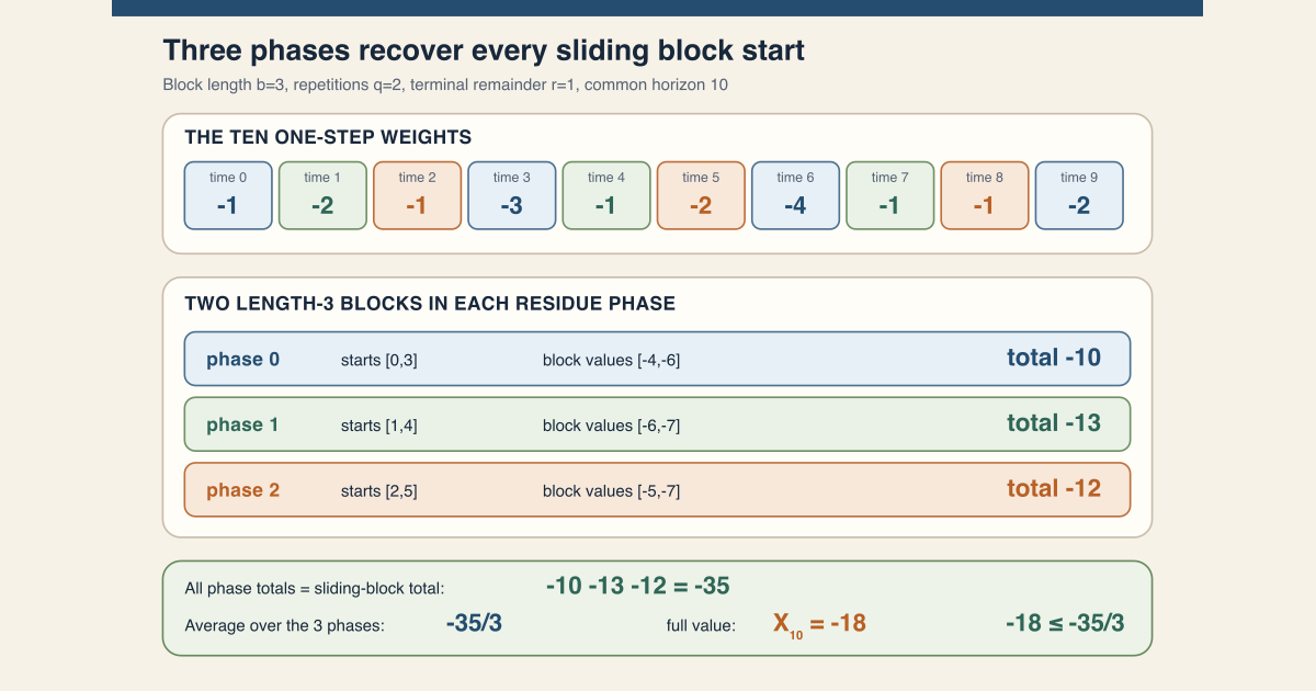
\[ \bigl(a(0),\ldots,a(9)\bigr) =(-1,-2,-1,-3,-1,-2,-4,-1,-1,-2). \]Set \(a(t)=-1\) for every \(t\ge10\), so this is a total nonpositive observable on the clock space.
Define the \(n\)-step process by adding the next \(n\) weights:
\[ X_n(t)=\sum_{j=0}^{n-1}a(t+j). \]This process is actually additive:
\[ X_{m+n}(t)=X_n(T^m t)+X_m(t). \]Equality is stronger than the shifted-subadditive inequality used by the project. Every displayed one-step weight is nonpositive, so every positive finite sum in this window is nonpositive too.
Choose block length \(b=3\), repetitions \(q=2\), and terminal parameter \(r=1\). The common theorem horizon is
\[ bq+b+r=3\cdot2+3+1=10. \]The usual Euclidean division also says \(10=3\cdot3+1\). The theorem uses only \(q=2\) middle blocks in every phase: the remaining full block is spread between the prefix and tail boundaries as the phase changes.
For a length-three block, the six sliding values are:
| block start | \(0\) | \(1\) | \(2\) | \(3\) | \(4\) | \(5\) |
|---|---|---|---|---|---|---|
| \(X_3(\text{start})\) | \(-4\) | \(-6\) | \(-5\) | \(-6\) | \(-7\) | \(-7\) |
Separate those starts by their residue modulo three:
| phase \(s\) | starts \(s+3j\) | block values | phase total |
|---|---|---|---|
| \(0\) | \(0,3\) | \(-4,-6\) | \(-10\) |
| \(1\) | \(1,4\) | \(-6,-7\) | \(-13\) |
| \(2\) | \(2,5\) | \(-5,-7\) | \(-12\) |
The three phase totals recover the same six starts exactly:
\[ -10-13-12=-35. \]Therefore their average is \(-35/3\). The full ten-step process value is
\[ X_{10}(0)=-18, \]and the finite phase estimate becomes the checkable inequality
\[ -18\le-\frac{35}{3}. \]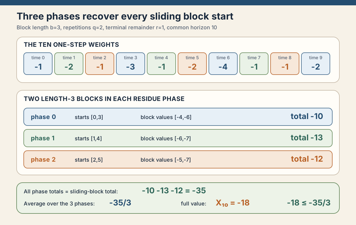
Why the sign and extra boundary block matter
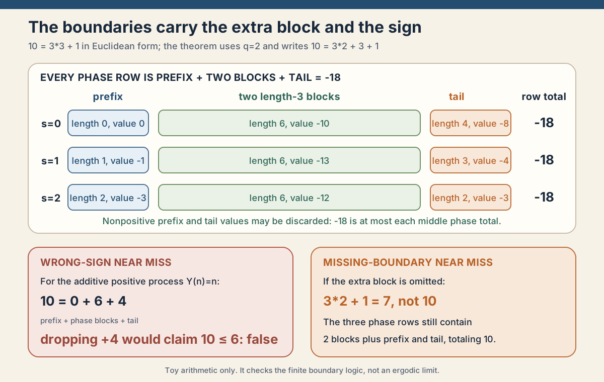
For each phase, the horizon ten splits into a prefix, two complete length-three blocks, and a tail:
| phase \(s\) | prefix length and value | middle length and value | tail length and value | sum |
|---|---|---|---|---|
| \(0\) | \(0,\ 0\) | \(6,\ -10\) | \(4,\ -8\) | \(-18\) |
| \(1\) | \(1,\ -1\) | \(6,\ -13\) | \(3,\ -4\) | \(-18\) |
| \(2\) | \(2,\ -3\) | \(6,\ -12\) | \(2,\ -3\) | \(-18\) |
All prefix and tail values are at most zero. Removing them makes the right-hand side larger, which preserves an upper bound. For example,
\[ -18=0+(-10)+(-8)\le-10. \]Now test the wrong sign. Let \(Y_n(t)=n\), the additive process generated by the positive one-step weight \(+1\). Phase zero gives
\[ Y_{10}(0)=10=0+6+4. \]Dropping the positive tail would claim \(10\le6\), which is false. Subadditivity alone does not justify boundary removal; positive-time nonpositivity supplies the needed direction.
There is a separate counting failure. Omitting the extra block would give
\[ bq+r=3\cdot2+1=7, \]but the prefix, two middle blocks, and tail still total ten. The horizon and the counted pieces would no longer describe the same object.
From the ledger to the general theorem
A block argument replaces the one-step map \(T\) by its \(b\)-step iterate \(T^b\). That replacement is useful because a single observation of the block observable \(X_b\) represents \(b\) original time steps. It is also dangerous: one powered orbit visits only the start times
\[ s,\ s+b,\ s+2b,\ \ldots, \]for one residue \(s\) modulo \(b\). Even if \(T\) is ergodic, \(T^b\) need not be ergodic. A proof cannot silently apply an ergodic theorem to the powered map and hope that the missing phases disappear.
Finite phase averaging repairs the combinatorics before any limit is considered. Here a phase is only a residue \(s\in\{0,\ldots,b-1\}\). It is not a complex angle, a random phase, an expectation, or a claim that a time average converges. For each phase, form a finite \(q\)-term Birkhoff sum under \(T^b\). Then sum those \(b\) sparse orbit sums. Every start time from \(0\) through \(bq-1\) appears exactly once, so the result is one ordinary \(bq\)-term Birkhoff sum under \(T\).
This chapter generalizes the ledger, proves the exact finite subadditive bound, audits every boundary, and maps the checked Lean module in source order. The immediate predecessor is Orbit-Majorant Centering for Subadditive Processes. The compact definition is the phase averaging glossary entry. The proof-to-prose companion is Average the Phases: Sliding-Block Bounds for Subadditive Cocycles in Lean.
Choose a route up
| Route | Begin | Destination |
|---|---|---|
| First encounter | Ten negative weights and three phases | Recompute every block, phase total, and boundary value |
| Arithmetic route | Why the sign and extra boundary block matter | Compare the valid bound with wrong-sign and missing-boundary near misses |
| Source route | The extra block is an arithmetic repair | Understand the corrected finite horizon |
| Lean translation route | Seven bridges | Match human statements, paper formulas, and exact declarations |
| Hands-on Lean route | Run the worksheet | Execute the complete integer ledger with only Std |
| Proof route | The four private proof engines | Rebuild the Lean architecture from raw algebra |
| API route | The eight public declarations | Read the exported interface in source order |
| Boundary route | Zero blocks and zero repetitions say different things | Separate vacuity from useful division |
| Assumption route | Wrapper fields are not proof dependencies | Audit signatures without erasing bundled facts |
| Integrity route | The exact stopping point | Block every convergence overread |
Learning objectives
By the summit, a reader should be able to:
- define a block phase as a residue modulo the block length;
- distinguish finite phase summation from expectation and ergodic averaging;
- expand a Birkhoff sum under the powered map \(T^b\);
- show that phase \(s\) samples starts \(s+bj\) for \(0\le j\lt q\);
- prove that all pairs \((s,j)\) cover exactly the starts below \(bq\);
- explain why commutativity is used when those terms are reordered;
- calculate the three phase rows for \(b=3\), \(q=2\), and \(r=1\);
- derive the exact prefix-block-tail identity;
- explain why the common horizon is \(bq+b+r\), not \(bq+r\);
- state the finite indexing inconsistency in Lalley’s displayed phase rows;
- distinguish the checked repair from another possible coherent repair;
- prove the raw terminal-remainder helper by induction on \(q\);
- derive the boundary-retaining phase theorem from two applications of shifted subadditivity;
- explain why the phase-zero proof must not invoke nonpositivity at time zero;
- prove that the two boundary lengths are positive when the sign theorem is actually used;
- sum the phase inequalities with
Finset.sum_le_sum; - convert a constant finite sum into multiplication by \(b\);
- distinguish the total multiplication theorem from the positive-block division theorem;
- explain why the multiplication theorem at \(b=0\) is vacuous;
- interpret the \(q=0\) theorem as a sign statement rather than a block average;
- reduce the construction at \(b=1\) to an ordinary Birkhoff sum;
- explain why \(r\) is unrestricted and may not be called a short remainder;
- use a process with \(X_0=1\) to refute an unnecessary time-zero premise;
- separate a candidate wrapper’s stored integrability from the fields used by a proof;
- separate the fields bundled in a cocycle from a separate generator-integrability witness;
- identify all eight public declarations in source order;
- identify all four private proof helpers in source order;
- identify the three named private smoke declarations;
- audit the empty matrix-index boundary;
- run the bounded
Stdworksheet on a normal macOS or Linux host; - reproduce the full project checks; and
- state why no Birkhoff, Kingman, Lyapunov, or Oseledets conclusion follows.
The common setup and notation ledger
Fix a state space \(\Omega\), a self-map \(T:\Omega\to\Omega\), and a real-valued process \(X_n(\omega)\) indexed by \(n\in\mathbb N\). The process is shifted-subadditive when
\[ X_{m+n}(\omega) \le X_n(T^m\omega)+X_m(\omega) \]for every \(m,n\) and \(\omega\). The shift matters because the later piece begins after the first \(m\) steps.
The finite Birkhoff sum of an observable \(g:\Omega\to M\) is
\[ \operatorname{BSum}(T,g,N,\omega) {} = \sum_{j=0}^{N-1}g(T^j\omega). \]Mathlib calls this birkhoffSum. Its definition and successor and
addition laws are the exact finite interfaces used by this module
(pinned Birkhoff-sum source). No convergence
theorem is present in that definition.
The parameters of the phase estimate have separate jobs:
| Symbol | Type | Job |
|---|---|---|
| \(b\) | natural number | block length and number of residue phases |
| \(q\) | natural number | complete \(b\)-blocks sampled in each phase |
| \(r\) | natural number | unrestricted extra terminal parameter |
| \(s\) | natural number with \(s\lt b\) | selected residue phase |
| \(\omega\) | element of \(\Omega\) | starting state |
The letter \(r\) is deliberately not called a Euclidean remainder. This module assumes neither \(r\lt b\) nor an equation that defines \(r\) by division. A later application may choose such an \(r\), but the finite API does not.
The sparse views that must be combined
For one fixed phase \(s\lt b\), the powered-map sum is
\[ \operatorname{BSum}(T^b,g,q,T^s\omega) {} = \sum_{j=0}^{q-1}g\bigl(T^{s+bj}\omega\bigr). \]The exponent identity behind this expansion is
\[ (T^b)^j(T^s\omega)=T^{bj+s}\omega. \]Lean reaches it through Function.iterate_mul and
Function.iterate_add_apply, whose pinned definitions and laws are
the local API authority (function iteration).
One phase is sparse. It sees one start in every group of \(b\) consecutive times. All phases together are complete. Every \(t\lt bq\) has a unique quotient \(j\lt q\) and residue \(s\lt b\) with \(t=bj+s\). Therefore
\[ \sum_{s=0}^{b-1} \operatorname{BSum}(T^b,g,q,T^s\omega) {} = \operatorname{BSum}(T,g,bq,\omega). \]This is a finite reindexing identity. It is valid in any additive commutative monoid because terms may be regrouped and reordered. It needs no measurable space, measure, integrability, probability, preservation, or ergodicity.
In Lean: seven bridges from the ledger to the project
The bridges below pair a human statement, paper mathematics, exact project syntax, and a token map. The standalone worksheet afterward executes the running integer example. The Mathlib-backed declarations are full project checks.
Bridge 1: write one sparse phase row
birkhoffSum (T^[b]) g q (T^[s] ω)birkhoffSumis Mathlib’s finite orbit-sum function.T^[b]is the \(b\)-fold iterate ofT, not exponentiation in a numeric ring.gis the observable; in the process theorem it becomesX b.qis the number of terms in this one phase row.T^[s] ωshifts the starting outcome into residue phases.
Bridge 2: reindex every phase into one sliding sum
sum_phase_birkhoffSum T g b q ωsum_phase_birkhoffSumis the first public declaration.bcontrols both the powered step and the number of phases.b * qis the number of chronological starts on the right.- The theorem assumes only
AddCommMonoidfor the values ofg; it uses no measure or limit.
Bridge 3: retain prefix and tail boundaries
hX.le_phase_birkhoffSum_add_boundaries b q r s hs ωhXis anIsIntegrableSubadditiveProcessCandidate T μ X.le_phase_birkhoffSum_add_boundariesuses only itsadd_lefield.hsprovess < b, so natural subtractionb + r - shas the intended length.- The nested iterate identifies the state at which the tail begins.
- No sign premise appears because both boundary values remain visible.
Bridge 4: remove boundaries with the correct sign
hX.le_phase_birkhoffSum hnonpos b q r s hs ωhnonposhas exact type∀ n, n ≠ 0 → ∀ ω, X n ω ≤ 0.- It controls positive horizons only; no claim about
X 0is required. - The theorem treats phase zero separately so it never asks
hnonposto prove a time-zero sign. - The wrong-sign process \(Y_n=n\) fails this premise and refutes the blocks-only conclusion numerically.
Bridge 5: sum all phase inequalities without dividing
hX.natCast_mul_le_birkhoffSum_phase_average hnonpos b q r ω(b : ℝ)in the theorem type casts the natural block length to a real scalar.natCast_mulin the name signals the multiplication form.Finset.sum_le_sumadds the phasewise inequalities internally.sum_phase_birkhoffSumchanges the right side from phase order to chronological order.- This theorem remains formally true at
b = 0, where it says only \(0\le0\).
Bridge 6: divide only after proving positive block length
hX.le_birkhoffSum_phase_average_div hnonpos b q r hb ωhb : b ≠ 0implies the real denominator is strictly positive.le_div_iff₀is the order equivalence used by the proof.- The division is by the number of phases \(b\), not by the number of block samples \(bq\).
- The separate theorem prevents the vacuous zero-block multiplication identity from being narrated as an average.
Bridge 7: specialize to the centered cocycle observable
Write \(\widetilde P_n\) for the cocycle’s log-positive norm observable after subtracting its one-step orbit majorant.
C.centeredLogPlusNormObservable_natCast_mul_le_birkhoffSum_phase_average b q r ωCis the bundled one-sided discrete matrix cocycle.C.basesupplies the map \(T\), although dot notation keeps it implicit in the call.centeredLogPlusNormObservable_add_lesupplies shifted subadditivity.centeredLogPlusNormObservable_nonpossupplies the sign at every horizon.- No separate probability, ergodicity, generator-integrability, or nonempty matrix-index argument appears.
Type the three-phase ledger yourself with Lean and Std
The following file imports only Lean’s small Std library. It
constructs the ten integer weights, enumerates phase starts, computes block and
boundary ledgers, checks the rational phase average, and executes both near
misses. It does not import Mathlib or define a project
birkhoffSum.
Save this exact text as
/tmp/SubadditivePhaseAveragingTutorial.lean:
import Std

namespace SubadditivePhaseAveragingTutorial

def weight : Nat → Int
  | 0 => -1
  | 1 => -2
  | 2 => -1
  | 3 => -3
  | 4 => -1
  | 5 => -2
  | 6 => -4
  | 7 => -1
  | 8 => -1
  | 9 => -2
  | _ => -1

def process (n start : Nat) : Int :=
  ((List.range n).map fun j => weight (start + j)).sum

def blockLength : Nat := 3
def repetitions : Nat := 2
def remainder : Nat := 1

def horizon : Nat :=
  blockLength * repetitions + blockLength + remainder

def phaseStarts (s : Nat) : List Nat :=
  (List.range repetitions).map fun j => s + blockLength * j

def phaseBlockValues (s : Nat) : List Int :=
  (phaseStarts s).map fun start => process blockLength start

def phaseTotal (s : Nat) : Int :=
  (phaseBlockValues s).sum

def phaseTotals : List Int :=
  (List.range blockLength).map phaseTotal

def slidingBlockValues : List Int :=
  (List.range (blockLength * repetitions)).map fun start =>
    process blockLength start

def slidingTotal : Int :=
  slidingBlockValues.sum

def prefixValue (s : Nat) : Int :=
  process s 0

def tailLength (s : Nat) : Nat :=
  blockLength + remainder - s

def tailStart (s : Nat) : Nat :=
  s + blockLength * repetitions

def tailValue (s : Nat) : Int :=
  process (tailLength s) (tailStart s)

def boundaryLedger (s : Nat) : List Int :=
  [prefixValue s, phaseTotal s, tailValue s]

def phaseAverage : Rat :=
  (slidingTotal : Rat) / blockLength

def wrongSignProcess (n _start : Nat) : Int :=
  n

def wrongSignPhaseTotal : Int :=
  ((phaseStarts 0).map fun start =>
    wrongSignProcess blockLength start).sum

#eval (List.range horizon).map weight
#eval [horizon / blockLength, horizon % blockLength, repetitions]
#eval (List.range blockLength).map phaseStarts
#eval (List.range blockLength).map phaseBlockValues
#eval phaseTotals
#eval slidingBlockValues
#eval slidingTotal
#eval (List.range blockLength).map boundaryLedger
#eval process horizon 0
#eval phaseAverage
#eval (blockLength : Int) * process horizon 0 ≤ slidingTotal
#eval (process horizon 0 : Rat) ≤ phaseAverage
#eval [wrongSignProcess horizon 0, wrongSignPhaseTotal]
#eval wrongSignProcess horizon 0 ≤ wrongSignPhaseTotal
#eval [blockLength * repetitions + remainder, horizon]

example : horizon = 10 := by native_decide
example : phaseTotals = [-10, -13, -12] := by native_decide
example : slidingBlockValues = [-4, -6, -5, -6, -7, -7] := by
  native_decide
example : slidingTotal = -35 := by native_decide
example : (List.range blockLength).map boundaryLedger =
    [[0, -10, -8], [-1, -13, -4], [-3, -12, -3]] := by
  native_decide
example : process horizon 0 = -18 := by native_decide
example : phaseAverage = -(35 / 3 : Rat) := by native_decide
example : (blockLength : Int) * process horizon 0 ≤ slidingTotal := by
  native_decide
example : (process horizon 0 : Rat) ≤ phaseAverage := by native_decide
example : wrongSignProcess horizon 0 = 10 := by native_decide
example : wrongSignPhaseTotal = 6 := by native_decide
example : ¬ wrongSignProcess horizon 0 ≤ wrongSignPhaseTotal := by
  native_decide
example : blockLength * repetitions + remainder = 7 := by native_decide

end SubadditivePhaseAveragingTutorial
Run it on an ordinary Mac or Linux host with the pinned compiler, without
entering formalization/ and without invoking Lake:
source "$HOME/.elan/env"
elan run leanprover/lean4:v4.32.0 lean \
  /tmp/SubadditivePhaseAveragingTutorial.lean
The exact file above was executed successfully with Lean 4.32.0 and printed:
[-1, -2, -1, -3, -1, -2, -4, -1, -1, -2]
[3, 1, 2]
[[0, 3], [1, 4], [2, 5]]
[[-4, -6], [-6, -7], [-5, -7]]
[-10, -13, -12]
[-4, -6, -5, -6, -7, -7]
-35
[[0, -10, -8], [-1, -13, -4], [-3, -12, -3]]
-18
(-35 : Rat)/3
true
true
[10, 6]
false
[7, 10]
Read the second line as
[Euclidean quotient, Euclidean remainder, theorem repetitions].
The two true lines certify the integer multiplication bound and
the rational division bound. The false line is the wrong-sign
claim \(10\le6\), and [7, 10] contrasts the missing-extra-block
horizon with the checked one.
Resource profile: small standalone tutorial, local-safe. The
native_decide examples are kernel-checked proofs about this
concrete finite representation. They do not establish Mathlib’s generic
reindexing theorem or the matrix-cocycle specialization. Those exact
declarations use the Full
project checks below.
Revisit the exact three-phase horizon
For the running values \(b=3\), \(q=2\), and \(r=1\), the ordinary Euclidean quotient and remainder of the horizon are
\[ 10=3\cdot3+1. \]The theorem reserves one of those three full blocks for boundary motion. It uses \(q=2\) complete middle blocks in every row:
| phase \(s\) | prefix length | complete-block starts | tail length | row length |
|---|---|---|---|---|
| \(0\) | \(0\) | \(0,3\) | \(4\) | \(10\) |
| \(1\) | \(1\) | \(1,4\) | \(3\) | \(10\) |
| \(2\) | \(2\) | \(2,5\) | \(2\) | \(10\) |
Across the three rows, the six complete-block starts are exactly \(0,1,\ldots,5\). Prefix plus tail is always four, one full block plus the example’s Euclidean remainder \(1\). The general theorem does not require its parameter \(r\) to be a Euclidean remainder; that extra interpretation is specific to this ledger.
The generic arithmetic is the same:
\[ \begin{aligned} s+bq+(b+r-s) &= bq+b+r. \end{aligned} \]That equality is the geometry of the boundary-retaining theorem.
The extra block is an arithmetic repair
The extra \(b\) in \(bq+b+r\) is not proof slack. It is what lets every phase retain exactly \(q\) complete blocks while keeping both boundary lengths natural numbers.
The motivating phase display on page 2 of Lalley’s lecture notes is internally inconsistent as printed. In its row for phase \(s\), the right side contains \(n\) complete blocks of length \(m\), an initial segment of length \(s\), and a terminal segment of length \(k+m-s\). Those lengths total
\[ s+nm+(k+m-s)=(n+1)m+k, \]while the left side is labeled \(nm+k\). Across all \(m\) displayed rows, the one-step boundary occurrences total \(m(k+m)\), not the later printed count \(mk\). The checked Lean theorem keeps \(n\), renamed \(q\), full blocks per phase and therefore uses \((n+1)m+k\), renamed \(bq+b+r\), together with exactly \(nm=bq\) sliding-block starts. This is an explicit finite arithmetic repair of the displayed indices (Lalley, page 2).
There is another coherent repair: keep the horizon \(nm+k\) but use one fewer complete block in every phase. That choice would produce only \((n-1)m\) sliding starts. It is not the interface formalized here. The chapter does not determine the author’s intended edit. This finite counting discrepancy does not by itself contradict the asymptotic Kingman theorem, but the incompatible counts cannot be presented as an exact identity.
From one phase to a subadditive bound
Fix \(s\lt b\). Cut the common horizon into three consecutive pieces:
- a prefix of length \(s\);
- \(q\) complete blocks of length \(b\), beginning at \(T^s\omega\); and
- a terminal gap of length \(b+r-s\).
Repeated shifted subadditivity gives
\[ \begin{aligned} X_{bq+b+r}(\omega) &\le \operatorname{BSum}(T^b,X_b,q,T^s\omega) \\ &\quad+ X_{b+r-s}\bigl((T^b)^q(T^s\omega)\bigr) {}+X_s(\omega). \end{aligned} \]This inequality retains both boundaries. It consumes only the raw shifted-subadditive law. It neither assumes nor proves that any displayed function is integrable.
Now suppose only that the process is nonpositive at positive horizons:
\[ n\ne0\quad\Longrightarrow\quad X_n(\omega)\le0. \]For a positive phase \(s\), both boundary lengths are positive. The prefix is positive by definition, and \(s\lt b\) implies
\[ b+r-s\ge1. \]Both boundary values may therefore be discarded. Phase zero is subtler. Its prefix would be \(X_0(\omega)\), and the hypothesis says nothing about \(X_0\). The proof avoids introducing that term: it applies the terminal-remainder helper directly with remainder \(b+r\). Since a phase \(0\lt b\) exists only when \(b\gt0\), the terminal length \(b+r\) is positive and its value may be discarded.
The result for every actual phase is
\[ X_{bq+b+r}(\omega) \le \operatorname{BSum}(T^b,X_b,q,T^s\omega). \]This case split is the exact reason the theorem needs no premise \(X_0=0\).
Sum the phases, then divide only when legal
Sum the last inequality over all \(s\lt b\). The left side is constant in \(s\), so it becomes \(bX_{bq+b+r}(\omega)\). The right side collapses by the pure reindexing theorem:
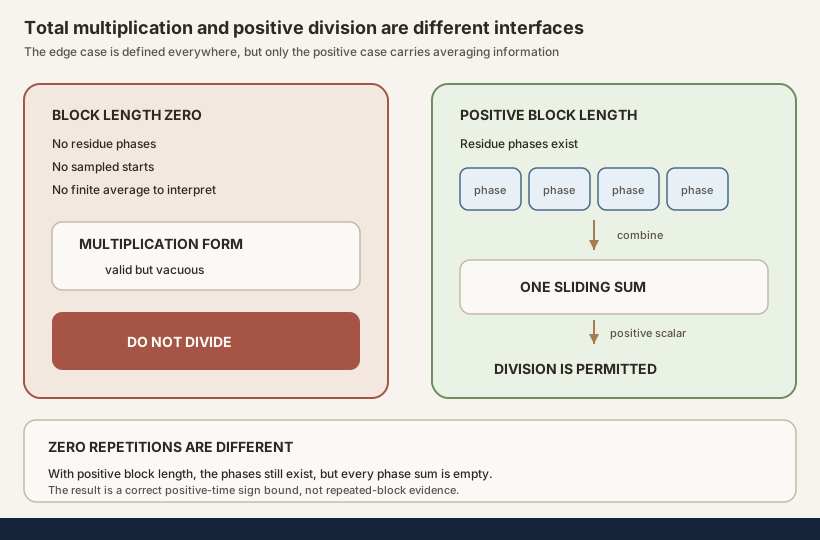
\[ bX_{bq+b+r}(\omega) \le \operatorname{BSum}(T,X_b,bq,\omega). \]In Lean, the real scalar is written (b : ℝ). This multiplication
form is total at \(b=0\). Both sides then reduce to zero, so the theorem says
only \(0\le0\). There are no phases, no samples, and no informative average.
For \(b\ne0\), the real cast of \(b\) is positive, and division preserves the inequality:
\[ X_{bq+b+r}(\omega) \le \frac{1}{b}\operatorname{BSum}(T,X_b,bq,\omega). \]The module exposes these as separate declarations because they carry different information at the boundary.
The four private proof engines
Private declarations do not appear in downstream APIs, but they expose the minimal mathematics. The module places four of them after the pure public reindexing theorem.
Private helper 1: le_blocks_add_remainder_of_add_le
This is the raw blocks-plus-terminal-remainder induction:
\[ X_{bq+r}(\omega) \le \operatorname{BSum}(T^b,X_b,q,\omega) {}+X_r\bigl((T^b)^q\omega\bigr). \]The base case \(q=0\) simplifies to reflexivity. At the successor step, peel
one \(b\)-block, apply the induction hypothesis at \(T^b\omega\), then use
birkhoffSum_succ’ and iterate_succ_apply. The helper
is local because the analogous engine in the predecessor module is private.
Private helper 2: le_phase_birkhoffSum_add_boundaries_of_add_le
This helper first cuts off the prefix \(s\), then invokes helper 1 on the
remaining \(bq+(b+r-s)\) steps. Natural subtraction is safe because
\(s\le b+r\), a consequence of \(s\lt b\). The result keeps both boundary
terms and uses only hadd.
Private helper 3: le_phase_birkhoffSum_of_add_le_nonpos
This helper adds positive-horizon nonpositivity. The s = 0 branch
uses helper 1 directly and drops only the positive terminal gap. The
s = s+1 branch uses helper 2 and drops two provably positive
gaps. This structure prevents an accidental use of the sign premise at time
zero.
Private helper 4: natCast_mul_le_birkhoffSum_phase_average_of_add_le_nonpos
The last engine applies helper 3 inside Finset.sum_le_sum, then
simplifies the constant sum with Finset.sum_const,
Finset.card_range, and nsmul_eq_mul. The public
sum_phase_birkhoffSum closes the right side. No integral or limit
appears.
The eight public declarations
The exported interface has eight declarations, listed below in their own source order. The complete source interleaving is public declaration 1, the four private helpers from the preceding section, then public declarations 2 through 8.
Declaration 1: sum_phase_birkhoffSum
For an additive commutative monoid \(M\), this theorem reindexes the double finite sum over phase and powered-map time as one base-map Birkhoff sum. It is the only public declaration before the private engines. The proof inducts on \(q\), extends every phase row by one term, uses the induction hypothesis on the old rectangle, and identifies the new row of \(b\) terms with the next length-\(b\) piece of the base sum.
Declaration 2: le_phase_birkhoffSum_add_boundaries
This candidate method exposes private helper 2. Its public receiver
hX is an integrable subadditive-process candidate, but the proof
projects only hX.add_le. The integrability field is present in the
signature and unused in the proof.
Declaration 3: le_phase_birkhoffSum
An explicit premise gives nonpositivity at every nonzero horizon. The theorem drops the prefix and tail without adding \(X_0=0\). It still takes the candidate wrapper, but its body uses only the wrapper’s shifted inequality and the explicit sign premise.
Declaration 4: natCast_mul_le_birkhoffSum_phase_average
This is the total multiplication form
\[ (b:\mathbb R)X_{bq+b+r}(\omega) \le \operatorname{BSum}(T,X_b,bq,\omega). \]It is valid at \(b=0\), where it is vacuous. The theorem does not claim that a zero-length block defines a useful phase average.
Declaration 5: le_birkhoffSum_phase_average_div
The division form adds exactly \(b\ne0\). Lean turns that natural-number fact
into positivity of the real denominator and applies le_div_iff₀.
The theorem adds no restriction on \(r\).
Declaration 6: centeredProcess_natCast_mul_le_birkhoffSum_phase_average
RMT-19 defined centeredProcess by subtracting the one-step orbit
majorant. Its residual is shifted-subadditive and nonpositive at every
positive horizon. Declaration 6 supplies those two checked facts to private
helper 4. No new \(X_0=0\), sign, or measure-preservation argument is needed.
The method still receives hX. Its signature therefore carries the
measurable space, measure, and stored integrability of the original candidate.
The phase-averaging proof does not consume those analytic fields.
Declaration 7: centeredProcess_le_birkhoffSum_phase_average_div
This is the positive-\(b\) division form for the centered process. Its only new explicit premise beyond the candidate is \(b\ne0\). It does not assert that the centered process has mean zero or that either normalized side converges.
Declaration 8: centeredLogPlusNormObservable_natCast_mul_le_birkhoffSum_phase_average
The final theorem specializes declaration 6’s algebra to a one-sided discrete
matrix cocycle. It takes the cocycle \(C\) directly, not the separate
generator-log-positive integrability witness hC. Its proof uses
the direct centered shifted-subadditivity and nonpositivity theorems.
The phrase “directly from \(C\)” does not mean an assumption-free signature.
The DiscreteMatrixCocycle structure already stores a
measure-preserving base and a measurable generator. Those fields remain
present but are not projected by this proof. The theorem also works for an
empty matrix index because it has no nonempty-index premise.
Wrapper fields are not proof dependencies
Formal statements can carry more structure than their proof bodies inspect. The distinction matters here.
| Layer | What the signature carries | What this proof consumes |
|---|---|---|
| Pure reindexing | A map, observable, and additive commutative monoid | Finite sums and iterate identities |
| Private raw helpers | A map and a real process | Shifted subadditivity; positive-time sign only where stated |
| Candidate methods | Measurable space, measure, all-horizon integrability, shifted subadditivity | The stored shifted inequality, plus explicit sign or prior centered laws |
| Cocycle method | Measure-preserving base and measurable matrix generator bundled in \(C\) | Direct finite centered subadditivity and sign laws |
It is correct to say that declaration 2’s proof does not use integrability. It
would be incorrect to say that declaration 2’s public signature has no
integrability-bearing object. It is correct to say that declaration 8 takes no
hC. It would be incorrect to say that its cocycle input stores no
measure preservation.
No declaration adds probability normalization or ergodicity. No proof applies a Birkhoff theorem to \(T^b\). The finite phase identity returns to an ordinary sum along \(T\), but turning that sum into a limit remains separate work.
Zero blocks and zero repetitions say different things
At \(b=0\), Finset.range b is empty, the right Birkhoff sum has
length \(0\cdot q=0\), and the left scalar is zero. Declaration 4 reduces to
\(0\le0\) for every \(q,r,\omega\). There is no phase \(s\lt0\), so the
single-phase theorems have no instance. Declaration 5 assumes \(b\ne0\), so it
has no \(b=0\) instance.
At \(q=0\), positive \(b\) still gives \(b\) genuine phases, but each powered-map Birkhoff sum is empty. The multiplication theorem becomes
\[ bX_{b+r}(\omega)\le0. \]After division, this reduces to \(X_{b+r}(\omega)\le0\), already supplied by the sign premise because \(b+r\gt0\). It is a correct boundary theorem, not a many-block averaging result.
At \(b=1\), there is one phase. The powered map is \(T\), and the phase sum is the ordinary \(q\)-term Birkhoff sum. The division theorem becomes
\[ X_{q+1+r}(\omega) \le \operatorname{BSum}(T,X_1,q,\omega). \]These three probes distinguish totalization, empty repetition, and the first informative block length.
A positive time-zero value is allowed
The named private smoke process lives on the one-point space:
\[ P_0(*)=1, \qquad P_n(*)=-n\quad\text{for }n\gt0. \]It is shifted-subadditive over the identity map. The source proves this as
positiveAtZeroProcess_add_le by separating the cases \(m=0\),
\(n=0\), and both positive. Over the zero measure, every horizon is integrable,
so positiveAtZeroCandidate packages the process.
This process refutes an unnecessary premise. It violates \(P_0=0\), yet its positive horizons are nonpositive and the checked phase-average theorem applies. With \(b=2\), \(q=3\), and \(r=1\), the source compiles
\[ 2P_9(*) \le \operatorname{BSum}(\operatorname{id},P_2,6,*). \]The left side is \(-18\), while the right side is \(-12\), so the checked inequality is strict. The example is a calibration of positive-time nonpositivity, not an equality theorem.
The three named private smoke declarations occur after the anonymous probes:
positiveAtZeroProcessdefines the values;positiveAtZeroProcess_add_leproves the shifted inequality; andpositiveAtZeroCandidatepackages zero-measure integrability and subadditivity.
The anonymous probes separately compile \(b=0\), \(q=0\), \(b=1\), the one-phase reindexing identity, and the empty matrix index.
Lean proofcraft
Induct on the rectangular direction
The reindexing theorem inducts on \(q\), not \(b\). Increasing \(q\) by one
adds one observation to every phase, which forms one new length-\(b\) row in
the ordinary Birkhoff sum. This matches Nat.mul_succ and
birkhoffSum_add directly.
Rewrite every phase row at once
simp_rw [birkhoffSum_succ] expands all powered-map sums inside
the outer finite sum. Then Finset.sum_add_distrib separates the
old rectangle from its new row.
Prove exponent alignment from library identities
The new row contains
\((T^b)^q(T^s\omega)\). The target contains \(T^{bq+s}\omega\). The proof uses
iterate_mul and two applications of iterate_add_apply,
with arithmetic closed by omega. It does not rely on visual
similarity of exponent notation.
Generalize the sample in block induction
The terminal-remainder helper applies its induction hypothesis at
\(T^b\omega\), so the induction begins with generalizing ω. Without
that generalization, the hypothesis is fixed at the wrong starting state.
Make the phase-zero boundary a separate branch
A uniform call to the boundary-retaining theorem would introduce \(X_0\) at phase zero. Since the sign premise covers only positive horizons, the proof cases on \(s\). This is theorem design encoded as proof structure.
Let multiplication remain total
The raw averaged inequality does not divide. Only the public division theorem converts \(b\ne0\) into a positive real denominator. This keeps the useful zero-safe statement while making its vacuity explicit.
Common wrong turns
Keeping \(bq+r\) while retaining \(q\) blocks in every phase
The prefix and tail then do not fit. Either add the missing block, as this module does, or reduce the number of complete blocks. Do not combine one choice’s left side with the other’s right side.
Calling \(r\) a short remainder
No theorem states \(r\lt b\). The name “terminal parameter” is accurate until a separate quotient-and-remainder choice supplies the inequality.
Applying nonpositivity to \(X_0\)
The hypothesis explicitly excludes zero. The phase-zero branch is designed to avoid that application.
Dividing the \(b=0\) theorem
The multiplication form is valid but vacuous. Real division by the zero cast would not recover a meaningful estimate, so the division theorem requires \(b\ne0\).
Treating \(q=0\) as evidence from repeated blocks
Every block sum is empty. The remaining statement is the positive-time sign law in another form.
Erasing wrapper fields from prose
Unused fields are still present in a receiver type. Report both the public signature and the narrower proof dependency.
Adding a generator-integrability witness to the cocycle theorem
The pointwise centered laws already live on \(C\). A separate hC
would strengthen the API without serving the proof.
Assuming ergodicity passes to \(T^b\)
It does not in general. Phase reindexing is finite and does not need the false shortcut.
Reading the word “average” as a limit
For positive \(b\), division by \(b\) averages finitely many phase inequalities. It says nothing about \(q\to\infty\).
Upgrading an upper bound to equality
Equality holds for some normalized additive examples, but not for the positive-time smoke process: Exercise 34 computes the strict inequality \(-18\lt-12\). General shifted subadditivity can lose slack at every cut.
Forty solved exercises
The exercises move from finite arithmetic to theorem design. Every answer is included so the chapter can be used without a separate solution manual.
Base camp: see the finite grid
Exercise 1: define a phase without metaphor
What is a phase in this chapter?
Solution. For block length \(b\), a phase is a natural number \(s\) with \(s\lt b\). It selects the residue class of block starts congruent to \(s\) modulo \(b\). It is not a complex phase, a random variable, or an asymptotic average.
Exercise 2: list one powered orbit
Let \(b=3\), \(q=2\), and \(s=2\). Which original-time starts occur in the powered-map Birkhoff sum?
Solution. The starts are \(s+bj\) for \(j=0,1\), hence \(2,5\). The sum is \(\operatorname{BSum}(T^3,g,2,T^2\omega)\), and its two summands are \(g(T^2\omega)\) and \(g(T^5\omega)\).
Exercise 3: flatten the three-phase grid
List all starts for \(b=3\) and \(q=2\).
Solution. Phase zero gives \(0,3\); phase one gives \(1,4\); and phase two gives \(2,5\). Reordering these six starts gives \(0,1,\ldots,5\), exactly the range below \(bq=6\).
Exercise 4: prove uniqueness of a start
Why can two distinct pairs \((s,j)\) and \((s',j')\), with \(s,s'\lt b\), not represent the same start \(bj+s=bj'+s'\)? Assume \(b\gt0\).
Solution. Reducing both sides modulo \(b\) gives \(s=s'\), because both are canonical residues below \(b\). Subtracting the common residue gives \(bj=bj'\), and cancellation by positive \(b\) gives \(j=j'\). Thus the phase grid has no duplicates.
Exercise 5: inspect block length zero
What does sum_phase_birkhoffSum say at \(b=0\)?
Solution. The outer phase range is empty, so its sum is zero. The target Birkhoff sum has length \(0\cdot q=0\), so it is also zero. The identity is valid as \(0=0\), but there are no phases to interpret.
Exercise 6: inspect zero repetitions
What does the same identity say at \(q=0\)?
Solution. Every powered-map Birkhoff sum has zero terms, so every summand is zero. The target has length \(b\cdot0=0\). Both sides are zero for every block length.
Exercise 7: inspect block length one
Simplify the phase identity when \(b=1\).
Solution. There is only phase zero, \(T^1=T\), and \(T^0\omega=\omega\). The left side is therefore \(\operatorname{BSum}(T,g,q,\omega)\), which equals the right side because \(1\cdot q=q\).
Exercise 8: verify the common horizon
For arbitrary \(s\lt b\), add the prefix, complete-block, and terminal lengths.
Solution. Their sum is
\[ s+bq+(b+r-s)=bq+b+r. \]The \(s\) terms cancel. The result is independent of phase, which is why all phase inequalities can have the same left side.
Exercise 9: find both boundaries in the worked example
For \(b=3,q=2,r=1,s=2\), what are the boundary lengths and total length?
Solution. The prefix length is \(2\). The terminal length is \(b+r-s=3+1-2=2\). The two complete blocks contribute \(6\), so the total is \(2+6+2=10\).
Exercise 10: explain why commutativity appears
Why does the reindexing theorem assume an additive commutative monoid rather than only an additive monoid?
Solution. The phase sum orders terms first by residue \(s\), then by block counter \(j\). The target orders them by chronological time \(bj+s\). Passing between these orders permutes summands. Commutativity makes the value independent of that permutation.
Mid-mountain: rebuild the private engines
Exercise 11: prove the block helper’s base case
Set \(q=0\) in the terminal-remainder helper.
Solution. The left side is \(X_r(\omega)\). The Birkhoff sum has no terms, and \((T^b)^0\omega=\omega\), so the right side is \(0+X_r(\omega)\). The inequality is reflexive.
Exercise 12: identify the successor cut
How is the horizon \(b(q+1)+r\) rewritten before applying shifted subadditivity?
Solution. Natural arithmetic gives
\[ b(q+1)+r=b+(bq+r). \]The proof treats the first piece as one \(b\)-block and the later piece as the remaining \(bq+r\) steps beginning at \(T^b\omega\).
Exercise 13: justify generalizing ω
Why must the induction hypothesis work at a new sample?
Solution. After the first \(b\)-block is peeled off, the remaining process starts at \(T^b\omega\), not at \(\omega\). Generalizing the sample before induction lets the hypothesis be instantiated at that shifted state.
Exercise 14: derive the prefix cut
Rewrite \(bq+b+r\) as a prefix plus the rest for phase \(s\lt b\).
Solution. Since \(s\le b+r\),
\[ bq+b+r=s+\bigl(bq+(b+r-s)\bigr). \]Shifted subadditivity first pays \(X_s(\omega)\) and moves the remainder of the horizon to the state \(T^s\omega\).
Exercise 15: derive the boundary-retaining inequality
Combine the prefix cut with private helper 1.
Solution. Shifted subadditivity gives
\[ X_{bq+b+r}(\omega) \le X_{bq+(b+r-s)}(T^s\omega)+X_s(\omega). \]Apply helper 1 to the first term with starting state \(T^s\omega\) and remainder \(b+r-s\). Substitution gives exactly the powered block sum, the terminal boundary, and the prefix boundary.
Exercise 16: prove terminal positivity
Show that \(b+r-s\ne0\) whenever \(s\lt b\).
Solution. From \(s\lt b\), natural arithmetic gives \(s+1\le b\). Adding \(r\) yields \(s+1\le b+r\), so \(1\le b+r-s\). Hence the terminal length is positive and therefore nonzero.
Exercise 17: explain the phase-zero branch
Why is helper 2 not used uniformly at \(s=0\) when boundaries are discarded?
Solution. Helper 2 would include the prefix value \(X_0(\omega)\). The sign hypothesis applies only when its time index is nonzero. The proof instead uses the terminal-remainder helper directly, which introduces no zero-length prefix and needs to discard only \(X_{b+r}\).
Exercise 18: drop both positive-phase boundaries
Assume \(s\gt0\) and \(s\lt b\). Why are both boundary terms at most zero?
Solution. The prefix length \(s\) is nonzero by assumption. Exercise 16 shows that \(b+r-s\) is nonzero. The positive-horizon sign premise applies to both values at their respective states, so their sum is nonpositive and may be removed from the upper bound.
Exercise 19: sum the phase inequalities
Why does the left finite sum become \(bX_{bq+b+r}(\omega)\)?
Solution. The same process value appears once for every \(s\in\operatorname{range}(b)\). That finite set has cardinality \(b\). Summing a constant in an additive group gives \(b\) natural scalar copies, which for real numbers is multiplication by the cast \((b:\mathbb R)\).
Exercise 20: close the right side
What turns the sum of phasewise upper bounds into the sliding-block sum?
Solution. Apply sum_phase_birkhoffSum with observable
\(g=X_b\). It rewrites the sum of all \(q\)-term powered-map Birkhoff sums as
\(\operatorname{BSum}(T,X_b,bq,\omega)\).
High camp: audit the public API
Exercise 21: name declaration 1’s minimal structure
What assumptions does sum_phase_birkhoffSum actually state?
Solution. It needs a type \(\Omega\), a self-map \(T\), an observable into an additive commutative monoid, two natural numbers, and a sample. It states no measurable-space, measure, order, integrability, or dynamical premise.
Exercise 22: separate declaration 2’s signature and proof
Does le_phase_birkhoffSum_add_boundaries have an
integrability-free signature?
Solution. No. Its receiver is an
IsIntegrableSubadditiveProcessCandidate, which stores
all-horizon integrability as well as shifted subadditivity. The theorem’s body
uses only the add_le field. Both facts must be reported.
Exercise 23: locate the sign premise
Which generic public declarations explicitly take positive-time nonpositivity?
Solution. Declarations 3, 4, and 5 do:
le_phase_birkhoffSum,
natCast_mul_le_birkhoffSum_phase_average, and
le_birkhoffSum_phase_average_div. The boundary-retaining theorem
does not need the sign premise, and the centered variants obtain it from
RMT-19.
Exercise 24: explain declaration 4 at \(b=0\)
Why is it correct but uninformative?
Solution. Its left side is \(0\cdot X_r(\omega)=0\), and its right side is a zero-term Birkhoff sum, also zero. The theorem proves \(0\le0\). It does not average a nonempty family and gives no information about \(X_r\).
Exercise 25: derive declaration 5
How does \(b\ne0\) license division?
Solution. A nonzero natural \(b\) is positive. Its real cast is therefore
strictly positive. The ordered-field equivalence
le_div_iff₀ says that \(x\le y/b\) is equivalent to \(bx\le y\)
for a positive denominator, so declaration 4 supplies the required product
inequality.
Exercise 26: interpret \(q=0\) after division
Assume \(b\gt0\). What remains?
Solution. The Birkhoff sum has length \(b\cdot0=0\), so the division theorem says \(X_{b+r}(\omega)\le0\). Because \(b+r\gt0\), this is precisely an instance of the input sign premise.
Exercise 27: audit \(r\)
Can declaration 5 conclude that the terminal parameter is smaller than the block length?
Solution. No. The theorem quantifies over every natural \(r\) and contains no hypothesis \(r\lt b\). A Euclidean-remainder interpretation requires a separate definition and proof.
Exercise 28: audit the centered multiplication theorem
Which RMT-19 results power declaration 6?
Solution. The proof supplies
hX.centeredProcess_add_le as shifted subadditivity and
hX.centeredProcess_nonpos_of_ne_zero as positive-horizon
nonpositivity. It does not use the uniform sign theorem that would require
\(X_0=0\).
Exercise 29: audit the centered division theorem
What does declaration 7 add beyond declaration 6?
Solution. It adds only \(b\ne0\), converts that to positivity of the real cast, and divides. It adds no new measure-preservation, sign, probability, or ergodicity premise.
Exercise 30: audit the cocycle theorem
Why does declaration 8 take \(C\) rather than hC?
Solution. The proof needs only the pointwise theorems
C.centeredLogPlusNormObservable_add_le and
C.centeredLogPlusNormObservable_nonpos. Those are available from
the cocycle itself. The separate generator-log-positive integrability witness
would contribute no used fact.
Summit: countermodels, sources, and next theorems
Exercise 31: do not erase cocycle baggage
Does declaration 8 have a signature free of measure preservation?
Solution. Not literally. Its receiver \(C\) is a
DiscreteMatrixCocycle, whose structure stores a measure-preserving
base and a measurable generator. The proof does not project those fields, and
there is no additional preservation argument or premise.
Exercise 32: audit empty dimension
Why does the cocycle theorem remain available for index type
Empty?
Solution. The theorem assumes only Fintype and
DecidableEq for the matrix index, both of which exist for
Empty. It has no Nonempty premise. The source contains
an explicit empty-index smoke example.
Exercise 33: use the positive-time-zero countermodel
Which proposed premise does positiveAtZeroProcess refute?
Solution. It refutes the claim that phase averaging requires \(X_0=0\). The process has \(X_0=1\), is shifted-subadditive, and is nonpositive at every positive horizon. The compiled theorem still applies.
Exercise 34: check the smoke inequality numerically
Compute both sides for \(b=2,q=3,r=1\).
Solution. The horizon is \(2\cdot3+2+1=9\), so the left side is \(2P_9=2(-9)=-18\). The right side has six copies of \(P_2=-2\) along the identity orbit, so it is \(6(-2)=-12\). Thus the checked inequality is \(-18\le-12\), not equality. This also corrects the tempting but false shortcut of treating all positive-time values \(P_n=-n\) as additive across the exceptional time-zero boundary.
Exercise 35: audit Lalley’s displayed horizon
Count one phase row containing \(n\) blocks of length \(m\), prefix \(s\), and tail \(k+m-s\).
Solution. Its total is \(nm+s+(k+m-s)=(n+1)m+k\). Therefore it cannot be an exact decomposition of a left side labeled \(nm+k\). The Lean theorem keeps the \(n\) blocks and adds the missing \(m\) to the horizon.
Exercise 36: give the alternative repair
How could one retain the printed horizon \(nm+k\)?
Solution. Use only \(n-1\) complete \(m\)-blocks per phase. Then the prefix, \((n-1)m\) complete steps, and the \(k+m-s\) tail total \(nm+k\). That coherent theorem would reindex only \((n-1)m\) starts and is not RMT-20’s chosen API.
Exercise 37: reject a powered-map ergodic shortcut
Why does finite phase summation not prove that \(T^b\) is ergodic?
Solution. It proves only an equality of finite sums. Ergodicity is a measure-theoretic rigidity property of invariant sets or observables. The finite reindexing neither states nor implies it, and an ergodic map can have a nonergodic power.
Exercise 38: reject a Birkhoff conclusion
Why can declaration 5 not be followed immediately by “let \(q\to\infty\)”?
Solution. No theorem in the module establishes convergence of the normalized base-map Birkhoff sum, almost everywhere or otherwise. A valid passage also needs an exact normalization, measurable and integrable hypotheses, a pointwise or mean ergodic theorem, and control of how the horizon and \(r\) vary. None is supplied here.
Exercise 39: reject a Kingman conclusion
Which part of a Kingman proof has RMT-20 formalized?
Solution. It formalizes a finite upper-estimate ingredient: align all block phases and bound one nonpositive shifted-subadditive process value by a sliding finite block sum. It does not prove the limsup passage, the complementary lower estimate, invariance or constancy of a limit, or identification with an expected rate.
Exercise 40: design the next finite layer
What should precede any full subadditive ergodic theorem next?
Solution. The dependency-ordered next step is finite interval packing: select an ordered disjoint family of favorable intervals, prove its coverage and gap bookkeeping, and derive the complementary finite lower-estimate inequality. That combinatorics should remain independent of measure theory. Only afterward should a precise maximal inequality and almost-everywhere limit theorem be designed.
Full project checks
The local worksheet checks the designed ten-step ledger only. The following two probes inspect the actual Mathlib-backed module and its centering predecessor. Install the repository’s pinned dependencies first; these checks may require substantial disk space and memory.
The eight public phase-averaging declarations
The authoritative source is
formalization/NonlinearDynamics/Random/RandomCocycles/SubadditivePhaseAveraging.lean.
Place this probe in a temporary project scratch file:
import NonlinearDynamics.Random.RandomCocycles.SubadditivePhaseAveraging

open NonlinearDynamics.Random.RandomCocycles

#check sum_phase_birkhoffSum
#check IsIntegrableSubadditiveProcessCandidate.le_phase_birkhoffSum_add_boundaries
#check IsIntegrableSubadditiveProcessCandidate.le_phase_birkhoffSum
#check IsIntegrableSubadditiveProcessCandidate.natCast_mul_le_birkhoffSum_phase_average
#check IsIntegrableSubadditiveProcessCandidate.le_birkhoffSum_phase_average_div
#check IsIntegrableSubadditiveProcessCandidate.centeredProcess_natCast_mul_le_birkhoffSum_phase_average
#check IsIntegrableSubadditiveProcessCandidate.centeredProcess_le_birkhoffSum_phase_average_div
#check DiscreteMatrixCocycle.centeredLogPlusNormObservable_natCast_mul_le_birkhoffSum_phase_average
The eight #check commands follow source order. They expose the
pure reindexing identity, two single-phase bounds, two generic all-phase
bounds, two centered-process wrappers, and the cocycle specialization.
Private proof helpers and smoke tests are intentionally absent from the
downstream API.
Full project check: exact repository module plus Mathlib. From the repository root:
cd formalization
lake env lean NonlinearDynamics/Random/RandomCocycles/SubadditivePhaseAveraging.lean
This checks the complete leaf with the repository’s pinned toolchain and dependencies.
cd formalization
lake env lean -DwarningAsError=true NonlinearDynamics/Random/RandomCocycles/SubadditivePhaseAveraging.lean
Resource note: this exact file uses the repository's
pinned Lean and Mathlib dependencies. Initial project setup can require
substantial disk space and build time. For a lightweight first step on
macOS or Linux, use the page's standalone Lean-core or Std
tutorial.
The centering predecessor that supplies the sign
The paired predecessor is
formalization/NonlinearDynamics/Random/RandomCocycles/SubadditiveCentering.lean.
Its relevant interface can be inspected with:
import NonlinearDynamics.Random.RandomCocycles.SubadditiveCentering

open NonlinearDynamics.Random.RandomCocycles

#check centeredProcess
#check IsIntegrableSubadditiveProcessCandidate.centeredProcess_nonpos_of_ne_zero
#check IsIntegrableSubadditiveProcessCandidate.centeredProcess_add_le
#check DiscreteMatrixCocycle.centeredLogPlusNormObservable
#check DiscreteMatrixCocycle.centeredLogPlusNormObservable_nonpos
#check DiscreteMatrixCocycle.centeredLogPlusNormObservable_add_le
The first candidate theorem supplies nonpositivity only at nonzero horizons, exactly the sign expected by phase averaging. The second supplies shifted subadditivity. The cocycle declarations provide the same two properties for the final specialization without adding a generator-integrability premise.
From the repository root, check this leaf with:
cd formalization
lake env lean NonlinearDynamics/Random/RandomCocycles/SubadditiveCentering.lean
cd formalization
lake env lean -DwarningAsError=true NonlinearDynamics/Random/RandomCocycles/SubadditiveCentering.lean
Resource note: this exact file uses the repository's
pinned Lean and Mathlib dependencies. Initial project setup can require
substantial disk space and build time. For a lightweight first step on
macOS or Linux, use the page's standalone Lean-core or Std
tutorial.
These commands do not replace the pending human mathematical, source,
accessibility, and editorial reviews. This page remains a public open working
note with pro_reviewed: false.
What the milestone establishes
| Question | Checked answer |
|---|---|
| Do all residue-phase block sums reindex to one sliding sum? | Yes, by a pure finite identity |
| What is the exact common horizon? | \(bq+b+r\) |
| Are prefix and terminal gaps retained first? | Yes |
| Which sign premise discards them? | Nonpositivity at every nonzero horizon |
| Is \(X_0=0\) needed? | No |
| Is \(r\lt b\) assumed? | No |
| Is the multiplication form valid at \(b=0\)? | Yes, vacuously |
| Does division require positive block length? | Yes, through \(b\ne0\) |
| What does \(q=0\) recover? | The already-known positive-time sign law |
| Does the candidate signature carry integrability? | Yes |
| Does the phase proof consume that integrability field? | No |
Does the cocycle theorem take hC? | No |
| Does its cocycle receiver already bundle preservation? | Yes |
| Is empty matrix dimension supported? | Yes |
| Is any ergodic or convergence theorem proved? | No |
The exact stopping point
Kingman’s original work supplies the asymptotic destination for subadditive stochastic processes (Kingman, 1968). Steele’s proof gives useful finite interval-decomposition context for the later lower estimate (Steele, 1989). RMT-20 proves neither source’s asymptotic conclusion.
The module and this chapter do not prove or define any of the following:
- \(r\lt b\) or any Euclidean-remainder interpretation of \(r\);
- a uniform bound on either boundary term;
- a uniform absolute-value or negative-tail bound for \(X_n\);
- time-zero normalization \(X_0=0\);
- a new integrability theorem for the phase sums;
- a new measure-preservation theorem;
- probability normalization of the measure;
- ergodicity, mixing, independence, or decay of correlations;
- ergodicity of \(T^b\);
- a pointwise Birkhoff ergodic theorem;
- a mean Birkhoff ergodic theorem;
- convergence of normalized Birkhoff sums;
- pointwise or almost-everywhere convergence of \(X_n/n\);
- convergence in \(L^1\), probability, measure, or distribution;
- a limsup passage from the finite upper bound;
- the full upper estimate in Kingman’s theorem;
- a maximal inequality;
- ordered disjoint-interval packing;
- the complementary finite lower estimate;
- an invariant limiting random variable;
- almost-everywhere constancy of a limit;
- identification of a samplewise limit with an integrated Fekete rate;
- permission to exchange a limit and an integral;
- Kingman’s subadditive ergodic theorem;
- a signed logarithmic matrix-growth process;
- control of contraction hidden by the log-positive envelope;
- invertibility of cocycle matrices;
- a top or lower Lyapunov exponent;
- the Furstenberg-Kesten random-matrix-product theorem;
- an Oseledets multiplicative ergodic theorem;
- an invariant filtration or splitting;
- a nonempty matrix index;
- a two-sided cocycle or negative-time dynamics;
- a stochastic-stability theorem; or
- any assertion that finite phase summation by itself creates an asymptotic average.
Random matrix products are a classical setting where an eventual growth theorem matters (Furstenberg and Kesten, 1960). The present cocycle observable is log-positive, so it controls expansion while clipping contraction. Renaming its finite phase bound as a signed Lyapunov result would erase that mathematical choice.
Where to continue
Orbit-Majorant Centering for Subadditive Processes is the immediate predecessor. It constructs the positive-time nonpositive residual used by the centered declarations here.
Finite Block Decomposition for Subadditive Processes proves the block-and-remainder inductions underneath the private phase helper.
The phase averaging glossary chapter is the compact definition, finite residue grid, and boundary reference. The orbit-majorant centering chapter explains the positive-horizon residual used in declarations 6 through 8. The Birkhoff sum chapter develops the finite orbit-sum convention.
Average the Phases: Sliding-Block Bounds for Subadditive Cocycles in Lean is the Development Notebook companion with the declaration-by-declaration implementation narrative and milestone audit.
The immediate successor is Finite Ordered Interval Packing for Nonpositive Subadditive Processes. It states interval order, coverage, gap, endpoint, empty-mark, and strictness conventions explicitly. The compact ordered interval packing chapter and the RMT-21 Development Notebook give the shorter routes. From the viewpoint of RMT-20, later Kingman layers still had to choose and prove their exact measurable, integrable, maximal-inequality, stationarity, and almost-everywhere hypotheses rather than infer a limit from the shape of this finite formula.
Subadditive Upper Limsup Bounds Before Kingman Convergence is the later upper-asymptotic consumer. It uses this finite phase estimate and ordinary-map Birkhoff convergence, and explicitly stops before a matching lower bound or a samplewise limit.
The Guarded Real-Liminf Bridge to Log-Positive Kingman Convergence is the much later project-local endpoint. It reaches almost-everywhere log-positive convergence only after the intervening upper-limsup, lower-deviation, boundedness, and liminf layers. That endpoint depends on this finite estimate; it does not turn the eight RMT-20 declarations into convergence theorems.
References
All links below were checked on 2026-07-21. The pinned local Mathlib checkout
at commit 81a5d257c8e410db227a6665ed08f64fea08e997 is the exact
authority for Lean declaration names and definitions.
Mathlib contributors.
Birkhoff sums,
Mathlib 4 documentation. The pinned
definition and finite laws
define birkhoffSum and prove its zero, one, successor, and
addition identities. RMT-20 uses these finite laws only.
Mathlib contributors. Function iteration, Mathlib 4 documentation. The pinned iterate definitions and addition and multiplication laws justify the conversion from a powered-map phase term to its original-time start.
Steven P. Lalley. Kingman’s Subadditive Ergodic Theorem, University of Chicago lecture notes, 3 pages, undated, accessed 2026-07-21. Page 2 motivates phase averaging to avoid assuming that powers of an ergodic map remain ergodic. Its displayed phase rows contain the finite horizon and boundary-count inconsistency audited explicitly in this chapter. The notes are a teaching source, not the primary source for Kingman’s theorem and not a Lean dependency.
J. F. C. Kingman. The ergodic theory of subadditive stochastic processes, Journal of the Royal Statistical Society: Series B 30(3), 499-510, 1968. This primary source supplies the asymptotic subadditive-ergodic destination. RMT-20 proves only a finite upper-bound ingredient.
J. Michael Steele. Kingman’s subadditive ergodic theorem, Annales de l’Institut Henri Poincaré, Probabilités et Statistiques 25(1), 93-98, 1989. This proof-lineage source uses finite interval decompositions in a full proof. It motivates the separate interval-packing successor but is not an upstream theorem imported here.
Harry Furstenberg and Harry Kesten. Products of Random Matrices, The Annals of Mathematical Statistics 31(2), 457-469, 1960. This primary source motivates the random-matrix-product destination. No samplewise growth theorem from that paper is claimed or formalized in RMT-20.
The exact upstream Lean revision audited for this chapter is Mathlib commit
81a5d257,
the revision pinned by formalization/lake-manifest.json.