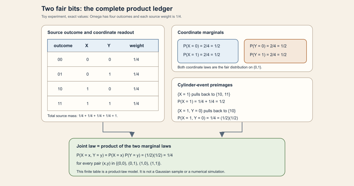
Four outcomes are enough to expose nearly every logical seam in a finite product probability space. We will compute all four rows, both coordinate laws, two event preimages, and the complete joint law. Only after those numbers are visible will we replace the bits by complex Gaussian coordinates.
That order matters. A product law is not a slogan saying that variables feel unrelated. It is a precise statement about the probability of every suitable coordinate event. In a four-row experiment, we can check the statement one cell at a time. In a continuous Gaussian field, Lean records the same idea through measures, measurable maps, exact laws, and mutual independence.
The word field here means a finite indexed family of random variables. It does not mean a continuum Gaussian process, an algebraic field, or a quantum field. The index type may later label upper-triangular matrix positions, but no matrix ensemble is defined in this chapter.
Base camp: two fair bits with no hidden rows
Let the sample space, the set of possible outcomes, be
\[ \Omega=\{00,01,10,11\}. \]Give every outcome weight \(1/4\). The resulting probability measure \(P\) has total mass
\[ P(\Omega)=\frac14+\frac14+\frac14+\frac14=1. \]Define two coordinate readouts:
\[ X(uv)=u,\qquad Y(uv)=v. \]For example, \(X(10)=1\) and \(Y(10)=0\). Each coordinate is a random variable : a measurable map from the outcome space to a value space. In this finite worksheet every subset is declared measurable, so measurability is automatic. In the continuous setting later, it will not be automatic.
Here is the complete experiment. There are no unlisted outcomes and no fitted or simulated values.
| source outcome \(\omega\) | \(X(\omega)\) | \(Y(\omega)\) | \(P(\{\omega\})\) |
|---|---|---|---|
| \(00\) | \(0\) | \(0\) | \(1/4\) |
| \(01\) | \(0\) | \(1\) | \(1/4\) |
| \(10\) | \(1\) | \(0\) | \(1/4\) |
| \(11\) | \(1\) | \(1\) | \(1/4\) |
The law or probability distribution of \(X\) collects source weights with the same \(X\)-value:
\[ \begin{aligned} P(X=0)&=P(\{00,01\})=\frac24=\frac12,\\ P(X=1)&=P(\{10,11\})=\frac24=\frac12. \end{aligned} \]The same calculation gives
\[ P(Y=0)=P(Y=1)=\frac12. \]This is a real probability distribution with no density formula. A distribution is a measure; a density is only one possible description of some measures.
Pull an event back to the source
An event is a measurable set of outcomes. If we ask for the target condition \(X=1\), its preimage is the source event
\[ X^{-1}(\{1\})=\{10,11\}. \]Therefore
\[ P(X=1)=P(\{10,11\})=\frac12. \]If both coordinates are constrained, then
\[ \{X=1,\;Y=0\} =X^{-1}(\{1\})\cap Y^{-1}(\{0\}) =\{10\}, \]so
\[ P(X=1,Y=0)=P(\{10\})=\frac14. \]An event that constrains selected coordinates and leaves the others free is a cylinder event. The event \(X=1\) is a cylinder in this two-coordinate product because \(Y\) may be either \(0\) or \(1\).
The product statement, in four finite views
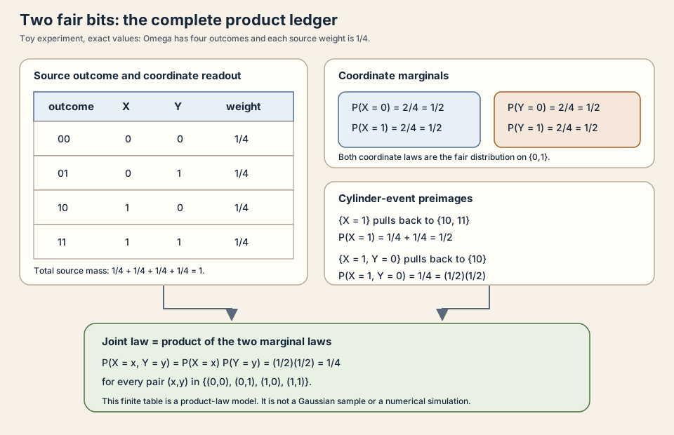
Let \(\mu_X\) and \(\mu_Y\) be the two coordinate laws. Each gives weight \(1/2\) to \(0\) and \(1/2\) to \(1\). Their product measure gives a rectangle \(A\times B\) the weight
\[ (\mu_X\otimes\mu_Y)(A\times B)=\mu_X(A)\mu_Y(B). \]For singleton rectangles in the running example,
\[ \begin{aligned} P(X=x,Y=y) &=P(X=x)P(Y=y)\\ &=\frac12\cdot\frac12\\ &=\frac14 \end{aligned} \]for every \(x,y\in\{0,1\}\). Because those four singleton rectangles exhaust the finite target, the complete joint law is the product law:
\[ \mathcal L_P(X,Y)=\mu_X\otimes\mu_Y. \]Here \(\mathcal L_P(X,Y)\) is the pushforward of \(P\) through \(\omega\mapsto(X(\omega),Y(\omega))\). Move each source weight to its observed pair, then combine weights that land at the same pair.
For this finite experiment, the same fact has four equivalent readings:
- every pair occurs in exactly one of four equally weighted source rows;
- every joint singleton has mass \(1/4\), the product of its marginal masses;
- the \(2\times2\) joint table has four entries, all \(1/4\); and
- the law identity is \(\mathcal L_P(X,Y)=\mu_X\otimes\mu_Y\).
The fourth form scales to continuous spaces. The first three make its meaning auditable before the notation becomes abstract.
Choose a route up
| Route | Begin with | Destination |
|---|---|---|
| First encounter | Two fair bits | Audit source weights, marginals, preimages, and the joint table |
| Dependence route | Three independence scopes | See why marginals, pairwise independence, and separate families are insufficient |
| Measure route | The exact product joint law | Understand Measure.pi and law-level factorization |
| Lean route | The standalone worksheet | Type finite code, then inspect the exact full project module |
| Geometry route | Real scaling | Track means, both variance functions, and independence under scaling |
| Matrix route | The ridge toward GUE | Identify every layer still missing before a named ensemble |
Learning objectives
By the summit, you should be able to:
- compute source weights, coordinate marginals, cylinder preimages, and the complete joint table for the four-outcome experiment;
- distinguish a coordinate law from the law of the complete indexed field;
- explain independence inside a complex coordinate and across complex coordinates as separate claims;
- distinguish pairwise independence from mutual independence;
- exhibit two separately independent real families whose paired complex variables are not independent;
- state the exact finite product law of an independent Cartesian complex Gaussian family;
- explain why ordinary coordinate measurability remains an explicit field;
- construct the canonical product probability space and its evaluation maps;
- derive the empty-index Dirac law without inventing an empty-matrix policy;
- type and run the finite
Stdworksheet without entering the project; - track coordinate means and both variances under real scaling;
- explain why general complex scaling can rotate an anisotropic Cartesian law out of the chosen independent axes; and
- list the representation and normalization decisions still required before a Gaussian unitary ensemble (GUE) law can be named.
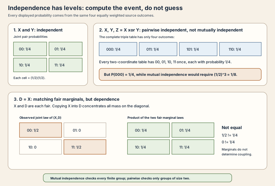
The dependence structure in one picture
Base camp: one outcome, many coordinates
Let \(\iota\) be a finite index type and \((\Omega,\mathcal F,P)\) a measured space. An indexed complex random field can be written in curried form as
\[ Z:\iota\longrightarrow\Omega\longrightarrow\mathbb C, \qquad Z_i(\omega)=Z(i)(\omega). \]For a fixed index \(i\), the map \(Z_i\) is one complex random variable. For a fixed outcome \(\omega\), the function
\[ i\longmapsto Z_i(\omega) \]is one complete field realization. Currying the arguments in the other order produces a single function-valued random variable
\[ \mathbf Z:\Omega\longrightarrow(\iota\to\mathbb C), \qquad \mathbf Z(\omega)(i)=Z_i(\omega). \]These views carry the same pointwise data, but they answer different questions. The coordinate view is natural for means, variances, and local laws. The function-valued view is natural for the joint law. A random matrix will eventually be assembled from the same pattern: one outcome produces all primitive coordinates at once.
Three layers must not be collapsed:
| Layer | Object | Question |
|---|---|---|
| Coordinate sample map | \(Z_i:\Omega\to\mathbb C\) | Is this map measurable, and what exact law does it have? |
| Field sample map | \(\mathbf Z:\Omega\to(\iota\to\mathbb C)\) | What joint value does one outcome produce? |
| Field law | \(\mathcal L_P(\mathbf Z)\) | How is probability distributed across all coordinate assignments? |
A table of coordinate means and variances describes only a small part of the third layer. The joint law must also say how the coordinates depend on one another.
Camp one: three independence scopes
The phrase “independent Gaussian coordinates” is dangerous until the unit of independence is named. This project needs three scopes.
Scope A: inside one complex coordinate
Write
\[ Z_i=X_i+iY_i, \]where \(X_i=\operatorname{Re}Z_i\) and \(Y_i=\operatorname{Im}Z_i\). An exact Cartesian complex Gaussian law states that \(X_i\) and \(Y_i\) have specified real Gaussian laws and are independent. This is a statement about two real axes inside one complex block.
It does not say anything about \(Z_i\) and \(Z_j\) for different indices.
Scope B: across complex blocks
The family-level statement says that the complex random variables
\((Z_i)_{i\in\iota}\) are mutually independent. In Lean this is iIndepFun Z P. It treats each entire complex coordinate as one block.
For measurable sets \(A_i\subseteq\mathbb C\), mutual independence gives the finite rectangle factorization
\[ P\!\left(\bigcap_{i\in\iota}\{\omega:Z_i(\omega)\in A_i\}\right) =\prod_{i\in\iota}P(Z_i\in A_i). \]The same principle extends from indicators of events to suitable products of measurable test functions. This is the content that later lets a joint law factor into coordinate laws.
Scope C: across two source families
Suppose a construction starts from two real families \((X_i)\) and \((Y_i)\). Knowing that the \(X_i\) are mutually independent and that the \(Y_i\) are mutually independent leaves all dependence between an \(X\)-coordinate and a \(Y\)-coordinate open.
Even adding same-index independence is not enough. Let \(A\) and \(B\) be independent standard real Gaussians and define, for two indices,
\[ X_1=A,\quad X_2=B, \qquad Y_1=B,\quad Y_2=A. \]Each source family is mutually independent. Each pair \((X_1,Y_1)\) and \((X_2,Y_2)\) also consists of independent standard Gaussians. Therefore each complex marginal
\[ Z_1=A+iB, \qquad Z_2=B+iA \]has the desired Cartesian complex Gaussian law. But
\[ Z_2=i\,\overline{Z_1}, \]so the two complex coordinates are deterministically related. Every local law is correct, while the field law is not a product.
This example is why the checked constructor begins with mutually independent pair-vectors \((X_i,Y_i)\). It puts the real and imaginary coordinate into one dependence block before asking for independence across indices.
Pairwise is still not mutual
Pairwise independence only checks one pair of indices at a time. Mutual independence checks every finite collection together. The distinction already appears in a three-variable discrete example. Let \(R\) and \(S\) be independent random signs, each equally likely to be \(-1\) or \(1\), and set \(T=RS\). Every pair among \(R,S,T\) is independent, but
\[ RST=1 \]always. The triple is not mutually independent.
Gaussian language does not automatically repair this gap. Pairwise independence can imply mutual independence for a jointly Gaussian vector, but separately declaring each marginal Gaussian does not prove that the complete vector is jointly Gaussian. The project records mutual independence directly instead of relying on an unstated joint-Gaussian hypothesis.
Camp two: the checked family bundle
The Lean structure makes the three required ingredients visible:
structure IndependentCartesianComplexGaussianFamily
    (Z : ι → Ω → ℂ) (m : ι → ℂ) (vRe vIm : ι → ℝ≥0)
    (P : Measure Ω) : Prop where
  measurable : ∀ i, Measurable (Z i)
  hasLaw : ∀ i,
    HasCartesianComplexGaussianLaw (Z i) (m i) (vRe i) (vIm i) P
  independent : iIndepFun Z P
The four parameter functions have different jobs:
Z iis the sample map for coordinate \(i\);m iis its complex mean;vRe iis the variance of its real part; andvIm iis the variance of its imaginary part.
Both variance functions take values in the nonnegative reals. The type prevents a negative variance while retaining zero as a legitimate degenerate case.
Why ordinary measurability is stored
A
measurable function
pulls every
measurable target event back to a measurable source event. The exact coordinate
predicate is built on HasLaw. Mathlib’s HasLaw contains an AEMeasurable
field, meaning that the map agrees almost everywhere with an ordinarily
measurable map. The exceptional outcomes lie inside a
null set
, a measurable set of probability zero.
Probability zero is not the same assertion as logical impossibility: a
nonempty set can have probability zero in a continuous space. Equality in law
should ignore null-set changes, so almost-everywhere measurability is the
correct law-level notion.
The family structure asks for ordinary Measurable (Z i) as separate data.
This stronger pointwise fact supports measurable coordinate transformations
and the canonical evaluation family. The theorem aemeasurable moves from the
strong field to the weaker consequence. It does not attempt the invalid reverse
direction.
Ordinary measurability implies almost-everywhere measurability under every measure. The reverse implication does not identify the original map on the exceptional set. The distinction is developed further in the almost-everywhere entry.
Coordinate consequences
For each index \(i\), the checked namespace exposes:
- exact real-part and imaginary-part Gaussian laws;
- the complex expectation \(\int Z_i\,dP=m_i\);
- real-part variance \(v_{\mathrm R,i}\);
- imaginary-part variance \(v_{\mathrm I,i}\);
MemLp (Z i) p Pfor every exponent \(p\ne\infty\), including Mathlib’s special \(p=0\) case; and- integrability of \(Z_i\).
The family also forces \(P\) to be a probability measure through the
normalization carried by iIndepFun. This remains true even when the index type
is empty.
These are coordinatewise theorems. They do not yet compute covariance matrices, densities, expectations of nonlinear field observables, or matrix trace moments.
Camp three: the exact product joint law
For finite \(\iota\), define the coordinate measure
\[ \mu_i =\Gamma^{\mathrm{cart}}_{m_i; v_{\mathrm R,i},v_{\mathrm I,i}}. \]The exact field law is
\[ \mathcal L_P(\mathbf Z) =\bigotimes_{i\in\iota}\mu_i. \]Mathlib writes the right side as
Measure.pi fun i ↦
  cartesianComplexGaussian (m i) (vRe i) (vIm i)
and the theorem
IndependentCartesianComplexGaussianFamily.jointHasLaw identifies the law of
fun omega i => Z i omega with that measure.
This theorem packages much more than a finite list of moments. It determines the probability of every measurable subset of the function space \(\iota\to\mathbb C\). The coordinate marginals can be recovered by evaluation, and the product form records the entire mutual-independence structure.
Nested product structure
Each complex coordinate measure is itself the image of a product of two real Gaussian measures. The field law therefore has a nested factorization:
\[ \bigotimes_{i\in\iota} \left( \gamma_{\operatorname{Re}m_i,v_{\mathrm R,i}} \otimes \gamma_{\operatorname{Im}m_i,v_{\mathrm I,i}} \right). \]On paper, reassociating this finite product shows that all real and imaginary axes are mutually independent under the exact family law. The current module does not expose that reassociation as a named theorem. Its checked public statement is the product of Cartesian complex blocks, which retains the hierarchy most useful for later matrix entries.
Exact law before qualitative joint Gaussianity
The theorem jointHasGaussianLaw forgets the explicit means and variance
functions and proves qualitative Gaussianity of the function-valued variable.
Mathlib reads \(\iota\to\mathbb C\) as a finite-dimensional real normed space,
so every continuous real-linear projection has a real Gaussian law.
That statement permits general finite-dimensional Gaussian arguments, but it
forgets the parameters. A matrix normalization depends on the actual functions
vRe and vIm, so the exact product law remains the authoritative interface
until the normalization ledger is complete.
Camp four: construct from independent real pair-vectors
The constructor of_independent_real_pair_laws accepts real maps
through their pair map
\[ Q_i(\omega)=(X_i(\omega),Y_i(\omega)). \]Its assumptions have a clean division of labor:
- each pair map \(Q_i\) is ordinarily measurable;
- each \(Q_i\) has the exact product of the requested real Gaussian laws;
- the family \((Q_i)_{i\in\iota}\) is mutually independent.
The second item contains within-coordinate independence. The third contains between-coordinate independence. Mapping every pair through \((x,y)\mapsto x+iy\) then produces the complex family without inventing any cross-family fact.
This design also explains why the constructor asks for a pair law rather than two marginal predicates. The pair law is a compact exact object that both fixes the two marginals and proves their internal independence.
Camp five: the canonical product probability space
An abstract family may live on any outcome space \(\Omega\). For existence proofs and reusable constructions, it is helpful to choose an outcome space whose points already are complete coordinate assignments:
\[ \Omega_{\mathrm{can}}=\iota\to\mathbb C. \]Define the probability measure
\[ P_{\mathrm{can}} =\bigotimes_{i\in\iota} \Gamma^{\mathrm{cart}}_{m_i; v_{\mathrm R,i},v_{\mathrm I,i}}. \]The project names this measure
cartesianComplexGaussianProductMeasure m vRe vIm. A sample
\(z\in\Omega_{\mathrm{can}}\) is a function, and the coordinate random
variables are evaluations
This construction has four checked layers:
| Declaration layer | Meaning |
|---|---|
| Probability instance | the finite product has total mass one |
| Evaluation law | \(E_i\) has exactly the requested Cartesian complex law |
| Evaluation independence | the family \((E_i)\) is mutually independent |
| Bundled family | measurable evaluations, exact laws, and independence are packaged together |
The evaluation map is ordinarily measurable because the measurable structure
on a function space is generated coordinatewise. Mathlib’s
measurePreserving_eval gives its exact pushforward law, while iIndepFun_pi
supplies mutual independence under the product measure.
Canonical does not mean unique
The canonical product space is a convenient realization of the joint law. It does not claim that every family with that law has the same underlying outcome space or the same pointwise samples. Two sample spaces may be very different while producing the same law on \(\iota\to\mathbb C\).
For distributional questions about the complete coordinate vector, the exact pushforward law is the invariant object. For constructions that need extra randomness or dynamical structure on \(\Omega\), the abstract family interface remains useful.
The empty-index boundary
If \(\iota\) has no elements, a function \(\iota\to\mathbb C\) still exists. In fact it is unique, because there is no index at which two such functions could differ. Call it \(z_{\varnothing}\).
The empty product measure has no coordinate factors to multiply. Its neutral probability-space interpretation is
\[ \bigotimes_{i\in\varnothing}\mu_i =\delta_{z_{\varnothing}}. \]Lean writes the unique function as fun i => isEmptyElim i. The theorem
cartesianComplexGaussianProductMeasure_eq_dirac_of_isEmpty proves
cartesianComplexGaussianProductMeasure m vRe vIm =
  Measure.dirac (fun i ↦ isEmptyElim i)
under Fintype ι and IsEmpty ι. The proof is Mathlib’s Measure.pi_of_empty.
This is not a technical afterthought. A finite construction that claims to cover arbitrary finite index types must say what happens at zero coordinates. The Dirac law is the correct neutral object for the scalar product space.
It does not choose a zero-dimensional matrix convention. A later matrix constructor may contain factors such as \(1/n\) or \(1/\sqrt n\), which are undefined at \(n=0\) unless an explicit policy is adopted. The empty scalar product and the empty matrix ensemble are different decision layers.
Camp six: real scaling preserves the Cartesian axes
For one coordinate, a real scalar \(c\) acts by
\[ Z\longmapsto cZ. \]If \(Z=X+iY\), then
\[ cZ=cX+i(cY). \]The chosen real and imaginary axes are unchanged. The mean and variances transform as
\[ m\longmapsto cm, \qquad v_{\mathrm R}\longmapsto c^2v_{\mathrm R}, \qquad v_{\mathrm I}\longmapsto c^2v_{\mathrm I}. \]HasCartesianComplexGaussianLaw.real_smul checks this exact single-coordinate
law. The family theorem scale permits a separate real scalar \(c_i\) at each
index and preserves all three structure fields:
- ordinary measurability survives a measurable deterministic map;
- each exact law receives the correct mean and squared variance factors; and
- mutual independence survives coordinatewise measurable transformations.
Negative scales are allowed. A zero scale turns that coordinate into the Dirac law at zero and leaves the family mutually independent.
Why the theorem does not accept an arbitrary complex scale
Let \(a,b\in\mathbb R\) and multiply by \(a+ib\). Then
\[ (a+ib)(X+iY) =(aX-bY)+i(bX+aY). \]The new real and imaginary coordinates mix both old axes. If \(X\) and \(Y\) are centered and independent with variances \(v_{\mathrm R}\) and \(v_{\mathrm I}\), paper calculation gives
\[ \begin{aligned} \operatorname{Var}(aX-bY) &=a^2v_{\mathrm R}+b^2v_{\mathrm I},\\ \operatorname{Var}(bX+aY) &=b^2v_{\mathrm R}+a^2v_{\mathrm I},\\ \operatorname{Cov}(aX-bY,bX+aY) &=ab\,(v_{\mathrm R}-v_{\mathrm I}). \end{aligned} \]Unless the original variances agree or the scale preserves the axes, the new coordinates can be correlated. The variable remains Gaussian as a real two-dimensional object, but it may no longer have an independent Cartesian decomposition in the displayed axes. These covariance formulas are textbook consequences, not declarations in the current Lean module. Restricting the checked scaling theorem to real scalars avoids claiming a rotation theorem that would need additional hypotheses and a new parameter transformation.
What the finite product law buys on paper
The exact product law supports several standard mathematical deductions. These deductions help orient future work, but only the items named in the Lean map below are currently formalized as project declarations.
Factorization of test functions
For bounded measurable functions \(f_i:\mathbb C\to\mathbb C\), mutual independence gives
\[ \mathbb E\!\left[\prod_{i\in\iota}f_i(Z_i)\right] =\prod_{i\in\iota}\mathbb E[f_i(Z_i)]. \]This identity is one analytic face of the product law. Choosing indicator functions recovers event factorization. Choosing exponentials gives a product characteristic function. The RMT-04 module does not add project-specific named theorems for these consequences.
Block-diagonal second-order structure
After centering, different complex blocks have zero cross-covariance whenever the required moments exist. Inside each block, the real and imaginary coordinates are independent and have their visible variances. Thus the real covariance matrix of the fully expanded finite vector is diagonal in the ordered Cartesian coordinate basis.
This statement depends on the full exact product structure. It would be false for the swapped-family counterexample even though every complex marginal is correct. The module exposes the hypotheses needed for a future covariance theorem but does not yet define that matrix or prove the diagonal formula.
Finite linear combinations
Every coordinate is integrable and belongs to every finite positive \(L^p\) class. For a finite index type, standard finite-sum arguments therefore give integrability of deterministic linear combinations. Qualitative joint Gaussianity additionally says that every continuous real-linear functional of the field has a real Gaussian law.
The current module proves coordinate MemLp, coordinate integrability, and
jointHasGaussianLaw. It does not name a complex linear-combination law with
an explicit resulting variance ledger.
In Lean: six bridges from the worksheet to the project
The bridges below pair a human sentence, paper mathematics, exact Lean syntax, and a token map. The first is a representation change. The remaining five name checked project interfaces.
Bridge 1: collect every coordinate into one value
fun ω i ↦ Z i ωfunbegins an anonymous function.ωis the source outcome andiis the coordinate index, in that order.↦separates inputs from output.Z i ωapplies the curried family first to the index and then to the outcome.- The result has type
Ω → (ι → ℂ). One outcome returns one function of the index.
Bridge 2: ask for mutual family independence
iIndepFun Z P- The initial lowercase
iiniIndepFunsignals an indexed family. Zhas curried typeι → Ω → ℂ.Pis the source measure. Independence is relative to a measure.- This is mutual independence, not merely one proposition for each pair of distinct indices.
Bridge 3: turn coordinate laws into one product joint law
hZ.jointHasLawThe exact theorem type is:
HasLaw (fun ω i ↦ Z i ω)
  (Measure.pi fun i ↦
    cartesianComplexGaussian (m i) (vRe i) (vIm i)) P
hZis evidence that the family satisfies the structure’s three obligations.HasLawis an exact pushforward-measure identity, not a moment approximation or a sampling command.Measure.piis Mathlib’s finite product measure here.m i,vRe i, andvIm iretain each coordinate’s mean and two Cartesian variances.- The theorem has a
[Fintype ι]assumption. Finiteness enters where this product-law interface needs it.
Bridge 4: ordinary measurability supplies the AE version
(hZ.measurable i).aemeasurablehZ.measurable iselects the ordinary measurability field at indexi.- The dot before
aemeasurableinvokes the implication from ordinary to almost-everywhere measurability. - The project theorem
IndependentCartesianComplexGaussianFamily.aemeasurablepackages the same step. - No converse is claimed, and no exceptional null set is promoted to an empty set.
Bridge 5: evaluate the canonical product sample
cartesianComplexGaussianProductMeasure_hasLaw_eval m vRe vIm icartesianComplexGaussianProductMeasureis the product measure onι → ℂ.hasLaw_evalsays the theorem concerns the evaluation mapfun z : ι → ℂ ↦ z i.- The companion theorem
cartesianComplexGaussianProductMeasure_iIndepFunproves mutual independence of all evaluations. - Together they produce
cartesianComplexGaussianProductMeasure_independentFamily, the canonical full structure.
Bridge 6: identify the empty product
cartesianComplexGaussianProductMeasure_eq_dirac_of_isEmpty m vRe vIm[IsEmpty ι]is the typeclass assumption saying no value of typeιexists.fun i ↦ isEmptyElim iis the unique function from that empty type into \(\mathbb C\).Measure.diracis the point-mass measure.- The theorem unfolds the canonical product and uses Mathlib’s
Measure.pi_of_empty. It does not divide by the index cardinality.
Try it locally: execute the four-row arithmetic
This first file imports only Lean’s small Std library. It deliberately models
finite rows and integer numerators, not measure theory and not Gaussian laws.
Save the following exact text as /tmp/FiniteProductTutorial.lean:
import Std

namespace FiniteProductTutorial

structure Outcome where
  x : Nat
  y : Nat
  deriving DecidableEq, Repr

def outcomes : List Outcome :=
  [⟨0, 0⟩, ⟨0, 1⟩, ⟨1, 0⟩, ⟨1, 1⟩]

def count (p : Outcome → Bool) : Nat :=
  (outcomes.filter p).length

def jointNumerators (first second : Outcome → Nat) : List Nat :=
  [count fun ω => first ω == 0 && second ω == 0,
   count fun ω => first ω == 0 && second ω == 1,
   count fun ω => first ω == 1 && second ω == 0,
   count fun ω => first ω == 1 && second ω == 1]

def parity (ω : Outcome) : Nat :=
  (ω.x + ω.y) % 2

def sourceLedger : List (Nat × Nat × Nat) :=
  outcomes.map fun ω => (ω.x, ω.y, 1)

def cylinderXOne : List (Nat × Nat) :=
  (outcomes.filter fun ω => ω.x == 1).map fun ω => (ω.x, ω.y)

def jointCylinderXOneYZero : List (Nat × Nat) :=
  (outcomes.filter fun ω => ω.x == 1 && ω.y == 0).map fun ω => (ω.x, ω.y)

#eval sourceLedger
#eval [count fun ω => ω.x == 0, count fun ω => ω.x == 1,
  count fun ω => ω.y == 0, count fun ω => ω.y == 1]
#eval cylinderXOne
#eval jointCylinderXOneYZero
#eval jointNumerators (fun ω => ω.x) (fun ω => ω.y)
#eval jointNumerators (fun ω => ω.x) (fun ω => ω.x)
#eval jointNumerators (fun ω => ω.x) parity
#eval jointNumerators (fun ω => ω.y) parity
#eval count fun ω => ω.x == 0 && ω.y == 0 && parity ω == 0

example : sourceLedger =
    [(0, 0, 1), (0, 1, 1), (1, 0, 1), (1, 1, 1)] := by
  decide

example : jointNumerators (fun ω => ω.x) (fun ω => ω.y) = [1, 1, 1, 1] := by
  decide

example : jointNumerators (fun ω => ω.x) (fun ω => ω.x) = [2, 0, 0, 2] := by
  decide

example : jointNumerators (fun ω => ω.x) parity = [1, 1, 1, 1] := by
  decide

example : jointNumerators (fun ω => ω.y) parity = [1, 1, 1, 1] := by
  decide

end FiniteProductTutorial
Type these commands on a normal macOS or Linux machine with Elan installed:
source "$HOME/.elan/env"
elan run leanprover/lean4:v4.32.0 lean /tmp/FiniteProductTutorial.lean
Standalone tutorial: Lean plus Std, suitable for a normal macOS or Linux
host. The command names the pinned compiler directly. It does not enter
the Lake project, restore Mathlib, or build the repository.
The file was executed with that exact command and printed:
[(0, 0, 1), (0, 1, 1), (1, 0, 1), (1, 1, 1)]
[2, 2, 2, 2]
[(1, 0), (1, 1)]
[(1, 0)]
[1, 1, 1, 1]
[2, 0, 0, 2]
[1, 1, 1, 1]
[1, 1, 1, 1]
1
Every count is a numerator over the four equally weighted rows:
[2, 2, 2, 2]gives both values of both marginals, each with mass \(2/4\);[(1, 0), (1, 1)]is the preimage of the cylinder \(X=1\);[(1, 0)]is the preimage of \(X=1,Y=0\);[1, 1, 1, 1]is the product joint table for \(X,Y\);[2, 0, 0, 2]is the dependent diagonal table for \(X,X\);- the next two product tables verify pairwise independence of \(X,Z\) and \(Y,Z\), where \(Z=X\mathbin{\mathrm{xor}}Y\); and
- the final
1says the all-zero triple occupies one of four rows, giving probability \(1/4\), not the mutual-product value \(1/8\).
The five example blocks are propositions checked by Lean’s kernel. They
certify list enumeration and natural-number arithmetic only. They do not
construct a probability measure, prove a theorem about Measure.pi, or show
that anything in the worksheet is Gaussian.
Try it in the repository: inspect the exact Gaussian interfaces
The authoritative source is
formalization/NonlinearDynamics/Random/ComplexGaussianFamilies.lean.
After installing the repository’s pinned dependencies, put this probe in a
temporary project scratch file:
import NonlinearDynamics.Random.ComplexGaussianFamilies

open MeasureTheory ProbabilityTheory
open scoped ENNReal NNReal ProbabilityTheory
open NonlinearDynamics.Random

#print IndependentCartesianComplexGaussianFamily
#check IndependentCartesianComplexGaussianFamily.measurable
#check IndependentCartesianComplexGaussianFamily.hasLaw
#check IndependentCartesianComplexGaussianFamily.independent
#check IndependentCartesianComplexGaussianFamily.aemeasurable
#check IndependentCartesianComplexGaussianFamily.of_independent_real_pair_laws
#check IndependentCartesianComplexGaussianFamily.jointHasLaw
#check IndependentCartesianComplexGaussianFamily.jointHasGaussianLaw
#check cartesianComplexGaussianProductMeasure
#check cartesianComplexGaussianProductMeasure_hasLaw_eval
#check cartesianComplexGaussianProductMeasure_iIndepFun
#check cartesianComplexGaussianProductMeasure_independentFamily
#check cartesianComplexGaussianProductMeasure_eq_dirac_of_isEmpty
#print displays the structure and its three separate proof obligations. Each
#check elaborates an existing declaration and reports its type.
These commands do not draw samples or estimate probabilities.
Full project check: exact repository module plus Mathlib. Check the authoritative module from the repository root with:
cd formalization
lake env lean NonlinearDynamics/Random/ComplexGaussianFamilies.lean
This command may compile substantial dependencies and therefore may require substantial disk space and memory.
cd formalization
lake env lean -DwarningAsError=true NonlinearDynamics/Random/ComplexGaussianFamilies.lean
Resource note: this exact file uses the repository's
pinned Lean and Mathlib dependencies. Initial project setup can require
substantial disk space and build time. For a lightweight first step on
macOS or Linux, use the page's standalone Lean-core or Std
tutorial.
The checked Lean map
The public interface is organized by layer:
| Layer | Declarations | Checked content |
|---|---|---|
| One complex variable | HasCartesianComplexGaussianLaw.real_smul | real scaling changes the mean linearly and both variances quadratically |
| Family definition | IndependentCartesianComplexGaussianFamily and its three fields | ordinary coordinate measurability, exact laws, mutual independence |
| Coordinate consequences | aemeasurable, isProbabilityMeasure, real_hasLaw, imag_hasLaw, mean_eq, real_variance_eq, imag_variance_eq, memLp, integrable | exact local probability and analytic facts |
| Pair-vector constructor | of_independent_real_pair_laws | exact product law inside each pair plus mutual independence across pairs |
| Family scaling | scale | coordinatewise real scaling preserves the complete bundle |
| Finite joint law | jointHasLaw, jointHasGaussianLaw | exact product law first, qualitative Gaussianity second |
| Canonical measure | cartesianComplexGaussianProductMeasure and its probability instance | a probability measure on the finite function space |
| Canonical coordinates | cartesianComplexGaussianProductMeasure_hasLaw_eval, cartesianComplexGaussianProductMeasure_iIndepFun, cartesianComplexGaussianProductMeasure_independentFamily | evaluation laws, mutual independence, complete bundled realization |
| Empty boundary | cartesianComplexGaussianProductMeasure_eq_dirac_of_isEmpty | the empty product is Dirac at the unique empty function |
The compiler-checked source is
formalization/NonlinearDynamics/Random/ComplexGaussianFamilies.lean. The
module makes no density, circularity, properness, matrix, spectral, or
asymptotic claim.
Validation boundary
The preceding repo-check block gives the copyable import, declaration probe,
exact module path, and full project command. The small standalone worksheet and the
Mathlib-backed repository module are intentionally separate validation layers.
The former checks four finite rows; the latter checks the actual Gaussian law,
measurability, mutual-independence, product-measure, and empty-index theorems.
The ridge toward a Gaussian matrix law
At the RMT-04 boundary, a finite independent complex field was useful raw material but not yet a matrix ensemble. A Hermitian matrix has two primitive coordinate roles and one determined region:
- diagonal entries are real;
- upper-triangular off-diagonal entries are complex;
- lower-triangular entries are determined by conjugating the upper triangle.
The third item means the lower-triangular entries are not independent primitive degrees of freedom. They are deterministically tied to the upper triangle by conjugation. One must first choose a primitive index set, sample independent values there, and then assemble the full matrix deterministically.
A dependence design is still required
One tempting design samples an independent real family for the diagonal and an independent complex family for the upper triangle. That still leaves dependence between those two families unstated. The same cross-family warning from this chapter returns at matrix scale.
A complete constructor must either:
- place all primitive blocks under one joint mutual-independence statement;
- construct them on a single canonical product space; or
- prove an equivalent product law joining the diagonal and off-diagonal families.
Naming both families “independent” separately is not enough.
The normalization ledger is still open
Before the words Gaussian unitary ensemble are attached to a Lean definition, the project must approve:
| Ledger slot | Missing decision |
|---|---|
| Matrix size | index type, dimension, and explicit \(n=0\) policy |
| Diagonal law | exact real mean and variance |
| Off-diagonal law | exact real-part and imaginary-part means and variances |
| Primitive independence | one joint statement across every sampled block |
| Hermitian reflection | the measurable assembly map into the matrix space |
| Dimension scaling | every factor involving \(n\) |
| Density convention | exponent and reference volume, if a density is used |
| Trace convention | raw trace or normalized trace |
| Spectral scale | intended order of eigenvalues |
RMT-04 fills the finite complex-family and canonical-product slots. It chooses none of the numerical values in this matrix ledger.
The later RMT-06 module now fills the ledger with diagonal variance \(1/n\), upper Cartesian variances \(1/(2n)\), a separate zero branch, and one product measure joining the diagonal and upper blocks. It then transports that measure through checked Hermitian assembly. Read Finite GUE from Independent Gaussian Coordinates for the completed bridge.
Construction is not invariance
Even after a matrix law is defined, unitary invariance is a separate theorem: conjugating the random matrix by every deterministic unitary matrix must leave its probability law unchanged. An entrywise product constructor does not prove that statement by name. The earlier random-matrix law layer supplies the language for it, and a future bridge must prove the equality of measures.
Common wrong turns
| Wrong turn | Why it fails | Correct layer |
|---|---|---|
| “The four-row worksheet is a Gaussian model” | its values are finite bits and its weights only teach exact product arithmetic | use the Mathlib-backed coordinate measures for Gaussian claims |
| “Every coordinate has the right law, so the field is independent” | marginals do not determine dependence | add iIndepFun or the exact product joint law |
| “Every pair is independent, so the family is mutually independent” | higher-order constraints can remain | state mutual independence directly |
| “The real family and imaginary family are each independent” | cross-family dependence is unproved | use independent pair-vectors or one global product law |
| “Each same-index real-imaginary pair is independent” | complex blocks can still share source variables | prove independence across the pair-vectors |
| “HasLaw makes every coordinate ordinarily measurable” | it carries only almost-everywhere measurability | store Measurable separately |
| “A product law is only a list of marginals” | it determines probabilities of all measurable field events | keep the joint map and Measure.pi identity |
| “Real scaling and complex scaling are the same theorem” | a complex scale mixes axes and can create covariance | keep the checked real-scalar theorem narrow |
| “The empty product decides the empty matrix” | matrix scaling may be undefined at zero dimension | choose the matrix policy separately |
| “An independent upper triangle is already GUE” | diagonal laws, scaling, assembly, and invariance remain | complete the matrix ledger and prove each bridge |
Exercises
Before leaving the four-row model, compute these without appealing to any Gaussian theorem:
- List the preimage of \(Y=0\) and add its source weights.
- Compute \(P(X=1\text{ or }Y=1)\) first by listing rows and then by inclusion-exclusion.
- Write all three \(2\times2\) pair tables for \(X\), \(Y\), and \(Z=X\mathbin{\mathrm{xor}}Y\). Explain why the triple constraint remains invisible in those tables.
- Change the coordinate laws to \(P(X=1)=1/3\) and \(P(Y=1)=1/4\). Under the product law, compute the four assignment weights and check that they sum to one.
- In the local Lean worksheet, add a
bothOnepredicate and prove withdecidethat its preimage has length one.
Summit register
The finite independent field layer is now exact. Every complex coordinate is ordinarily measurable, carries an exact Cartesian law with two visible variance parameters, and participates in one mutual-independence statement. For finite index types, the complete field map has the exact product of those coordinate laws. The same family hypotheses also yield qualitative joint Gaussianity, presented alongside the exact theorem. The project retains the parameter-rich product law as the primary interface while normalization data matters.
The canonical function-space measure realizes the law with measurable, mutually independent evaluation maps. Its empty-index case is the Dirac law at the unique empty assignment. Real coordinatewise scaling preserves the entire family contract and squares both variance functions.
This chapter’s summit is the finite Gaussian product law; the matrix ridge remains above it. No circular convention, dimension scale, diagonal law, primitive matrix index, Hermitian assembly, unitary invariance, eigenvalue law, trace expectation, or asymptotic statement has been selected or proved.
Where to continue
Use the Independent Cartesian complex Gaussian family entry for the compact definition and dependence checklist. The earlier Complex Gaussian Coordinates and Geometry chapter develops the one-coordinate law. The Gaussian Laws, Independence, and Normalization chapter supplies the real scalar and finite-product foundations.
Continue to Random Matrices: From Outcomes to Spectra for measurable matrix maps, Hermiticity, pushforward matrix laws, and trace observables. Read normalization convention before attaching any dimension-dependent scale.
Then use the Hermitian coordinate space and Finite Hermitian Matrices from Coordinates for the checked deterministic map from a real diagonal and complex strict upper triangle to a measurable Hermitian matrix. That map does not assert that the present complex family provides the diagonal coordinates, and it chooses no ensemble law.
Then continue to Finite GUE from Independent Gaussian Coordinates for the checked Wigner-scale coordinate product and matrix pushforward laws.
References
Mathlib contributors.
Independence of functions,
Mathlib 4 documentation. This official API defines IndepFun and
iIndepFun, preservation under measurable coordinate maps, finite product
joint laws, and independence of product-space evaluations.
Mathlib contributors.
Finite product measures,
Mathlib 4 documentation. This is the official source for Measure.pi,
measurePreserving_eval, probability preservation, and Measure.pi_of_empty.
Mathlib contributors.
Law of a random variable,
Mathlib 4 documentation. This documents the exact pushforward identity and
almost-everywhere measurability carried by HasLaw.
Mathlib contributors. Gaussian random variables and independence, Mathlib 4 documentation. This is the official source for qualitative joint Gaussianity of independent finite Gaussian families.
Olav Kallenberg. Foundations of Modern Probability, third edition, Springer, 2021. This standard monograph is cited for product probability spaces, random elements, and the measure-theoretic theory of independence.
N. R. Goodman. Statistical Analysis Based on a Certain Multivariate Complex Gaussian Distribution (An Introduction), The Annals of Mathematical Statistics 34(1), 152-177, 1963. This original article provides historical context for multivariate complex Gaussian laws; it does not fix the normalization or matrix representation used by this project.
Freeman J. Dyson. Statistical Theory of the Energy Levels of Complex Systems. I, Journal of Mathematical Physics 3, 140-156, 1962. This original article is cited for the historical symmetry-class motivation behind the later matrix program, not as a theorem about the present scalar product family.
The exact upstream Lean source audited for this chapter is Mathlib commit
81a5d257,
the revision pinned by formalization/lake-manifest.json.