Begin with two base points and two exact products
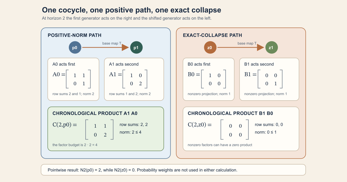
A matrix cocycle is a rule that reads a base state, applies the matrix stored there, moves the base state, and repeats. To make every symbol concrete, take the four-point base
\[ \Omega=\{p_0,p_1,z_0,z_1\}. \]Let the base map \(T:\Omega\to\Omega\) swap \(p_0\) with \(p_1\) and swap \(z_0\) with \(z_1\). Give each point mass \(1/4\). This uniform probability measure is preserved because \(T\) is a permutation, and every function on this finite discrete space is measurable.
The probability weights make the bundled cocycle legitimate, but none of the following pointwise arithmetic uses them. At the four base points, let the generator be
\[ \begin{aligned} A(p_0)&=A_0= \begin{bmatrix} 1&1\\ 0&1 \end{bmatrix}, & A(p_1)&=A_1= \begin{bmatrix} 1&0\\ 0&2 \end{bmatrix},\\[4pt] A(z_0)&=B_0= \begin{bmatrix} 1&0\\ 0&0 \end{bmatrix}, & A(z_1)&=B_1= \begin{bmatrix} 0&0\\ 0&1 \end{bmatrix}. \end{aligned} \]Regard these integer entries as complex numbers through the standard embedding. No genuinely complex arithmetic is needed for this example.
For a generator-presented cocycle, the two-step value is
\[ C(2,\omega)=A(T\omega)A(\omega). \]The matrix at the starting state acts first and therefore appears on the right.
The positive-norm sample
Starting from \(p_0\), the shear acts before the stretch:
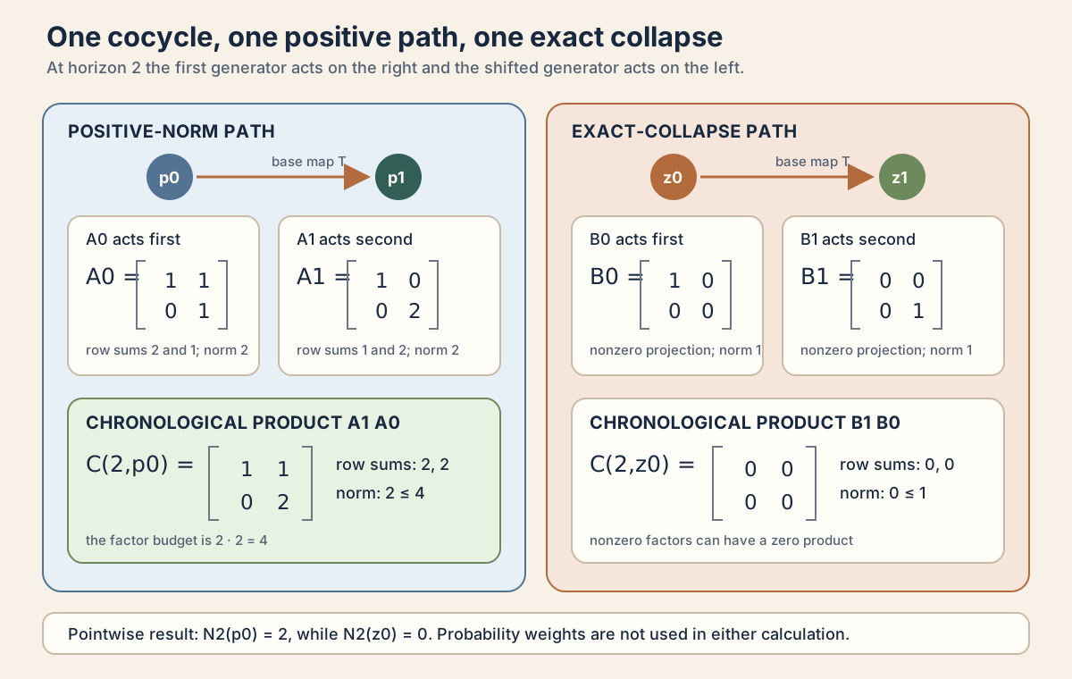
\[ \begin{aligned} C(2,p_0) &=A_1A_0\\ &= \begin{bmatrix} 1&0\\ 0&2 \end{bmatrix} \begin{bmatrix} 1&1\\ 0&1 \end{bmatrix}\\ &= \begin{bmatrix} 1&1\\ 0&2 \end{bmatrix}. \end{aligned} \]The two absolute row sums are \(2\) and \(2\). Hence its induced infinity operator norm, the maximum absolute row sum, is
\[ N_2(p_0)=\lVert C(2,p_0)\rVert_\infty=2. \]Each factor has norm \(2\), so the submultiplicative theorem gives the valid but non-sharp budget \(2\leq2\cdot2=4\).
The exact-collapse sample
Starting from \(z_0\), the first factor keeps only the first coordinate and the second keeps only the second coordinate:
\[ \begin{aligned} C(2,z_0) &=B_1B_0\\ &= \begin{bmatrix} 0&0\\ 0&1 \end{bmatrix} \begin{bmatrix} 1&0\\ 0&0 \end{bmatrix}\\ &= \begin{bmatrix} 0&0\\ 0&0 \end{bmatrix}. \end{aligned} \]Both \(B_0\) and \(B_1\) are nonzero and have norm \(1\), yet their product is zero. Thus
\[ N_2(z_0)=0\leq1\cdot1. \]This is the boundary that decides which logarithm the formalization needs.
Four finite-time values with different jobs
The target module defines the real norm observable
\[ N_k(\omega)=\lVert C(k,\omega)\rVert_\infty\in\mathbb R \]and the extended-real logarithm
\[ L_k(\omega) {} = \operatorname{ENNReal.log} \lVert C(k,\omega)\rVert_{\infty,e} \in\overline{\mathbb R}. \]Here \(\overline{\mathbb R}\), Lean’s EReal, is the real line
with bottom \(\bot=-\infty\) and top \(\top=+\infty\). The subscript \(e\)
only records the embedding of the nonnegative norm into the extended
nonnegative reals before taking the logarithm.
The immediate successor module defines a different real-valued function,
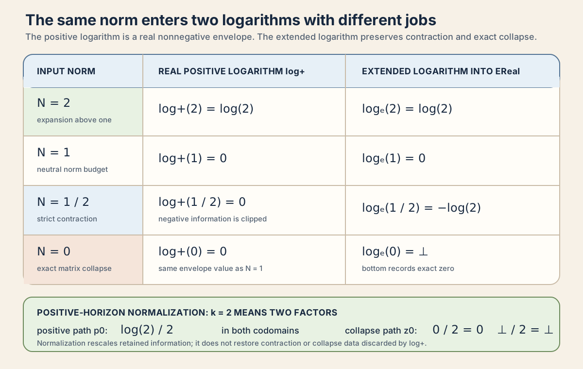
\[ G_k(\omega) {} = \log^+N_k(\omega) {} = \max\{0,\log N_k(\omega)\} \in\mathbb R. \]This positive logarithm is an integrability envelope. It keeps expansion above one and clips contraction, neutral norm, and exact collapse to zero (Mathlib contributors).
At a positive horizon, one can also inspect finite quotients
\[ \widehat G_k(\omega)=\frac{G_k(\omega)}{k}, \qquad \widehat L_k(\omega)=\frac{L_k(\omega)}{k}. \]The second quotient is extended-real arithmetic; dividing bottom by a positive
finite number leaves bottom
(Mathlib contributors). Neither quotient is defined by
NormObservables.lean, and one fixed quotient is not a limit.
For the two running samples at horizon two, the entire ledger is
| Quantity | Codomain | Positive path \(p_0\) | Collapse path \(z_0\) |
|---|---|---|---|
| Matrix value | \(M_2(\mathbb C)\) | \(\left[\begin{smallmatrix}1&1\\0&2\end{smallmatrix}\right]\) | \(0\) |
| \(N_2\) | \(\mathbb R\) | \(2\) | \(0\) |
| \(G_2=\log^+N_2\) | \(\mathbb R\) | \(\log2\) | \(0\) |
| \(L_2=\log_eN_2\) | EReal | \(\log2\) | \(\bot\) |
| \(\widehat G_2=G_2/2\) | \(\mathbb R\) | \(\frac12\log2\) | \(0\) |
| \(\widehat L_2=L_2/2\) | EReal | \(\frac12\log2\) | \(\bot\) |
The agreement on the positive path does not identify the two logarithms. Their zero policies are intentionally different.
Controlled near-misses
Using the ordinary real logarithm at zero
Lean’s total real logarithm satisfies
\(\operatorname{Real.log}(0)=0=\operatorname{Real.log}(1)\). Defining the
collapse-sensitive observable with Real.log would make the zero
matrix look indistinguishable from norm one. The target module therefore uses
ENNReal.log into EReal.
Calling the positive logarithm a signed growth rate
\(\log^+(1/2)=0\), \(\log^+(1)=0\), and \(\log^+(0)=0\). That loss is useful when proving integrability of a nonnegative upper envelope, but it cannot represent contraction or collapse. The later log-positive observable does not replace \(L_k\).
Dividing by the final factor index
Horizon two contains the factors with indices zero and one. Its normalizing factor is \(2\), not the last index \(1\). Dividing by one would double the positive path’s finite normalized value and would divide by zero at horizon one.
Treating time-zero totalization as growth information
Classically, \(X_0/0\) is not a normalized growth rate. Much later, the generic
real normalizedProcess defines the time-zero quotient to be zero
because Lean’s real division is total. Its own theorem says that this value
forgets \(X_0\) completely. Positive-time asymptotics may ignore that finite
prefix; this page must not reinterpret it as a meaningful zero-step rate.
Keep the formal layers separate
| Layer | Checked object or property | What it does not supply |
|---|---|---|
| Sample matrix | \(C(k,\omega)\) | A probability law or expectation |
| Target finite observable | \(N_k:\Omega\to\mathbb R\) | Integrability or normalized growth |
| Target extended observable | \(L_k:\Omega\to\overline{\mathbb R}\) | Almost-sure finiteness or an integral |
| Target regularity | Measurability of \(N_k\) and \(L_k\) | Integrability; measurable is weaker |
| Successor envelope | \(G_k=\log^+N_k:\Omega\to\mathbb R\) | Signed contraction or collapse data |
| Successor hypothesis | One-step integrability propagated to finite \(G_k\) | Automatic integrability from preservation |
| Probability law | A pushforward measure such as \((N_k)_*\mu\) | Not defined in either observable module |
| Positive-time normalization | A fixed quotient by \(k\) | A limit or Lyapunov exponent |
| Asymptotic theory | Kingman- or Oseledets-type conclusions under extra hypotheses | Not contained in this finite-time module |
The module
NonlinearDynamics.Random.RandomCocycles.NormObservables contains
fourteen public declarations. It proves finite pointwise algebra and
measurability only. Probability normalization, integrability, normalized
limits, Lyapunov exponents, and invariant splittings are separate later
decisions.
Choose a route up
| Route | Begin with | Destination |
|---|---|---|
| First encounter | Two exact products | Compute a positive norm and an exact collapse |
| Codomain route | Four finite-time values | Separate real norm, positive log, extended log, and normalized quotients |
| Near-miss route | Controlled near-misses | Audit zero policies, factor counts, and time-zero totalization |
| Norm route | Why this particular matrix norm | Compute the maximum absolute row sum and identify the active Lean scope |
| Measure route | Prove norm measurability from entries | Audit every closure step without assuming a hidden Borel instance |
| Endpoint route | Why the ordinary real logarithm is the wrong totalization | Preserve the difference between norm one and norm zero |
| Inequality route | The zero-safe subadditivity proof | Follow cocycle law, norm bound, monotonicity, and product-to-sum |
| Dimension route | Positive and empty dimensions | See exactly where nonempty coordinates are required |
| Lean route | Seven exact bridges | Translate human claims into exact project syntax |
| Hands-on route | Run the worksheet | Recheck the integer products and symbolic zero policies locally |
| Interface route | The complete fourteen-declaration map | Audit every public name, assumption, and output |
| Summit route | What has and has not been proved | Keep the finite-time boundary intact |
Learning objectives
By the summit, you should be able to reproduce both two-step products and every
row-sum norm; distinguish \(N_k\), \(G_k\), \(L_k\), and their positive-time
quotients by codomain and zero policy; explain why two nonzero factors may
produce bottom; read seven Lean bridges token by token; run the bounded
Std worksheet; reconstruct norm and log-norm measurability; follow
the zero-safe subadditivity proof; audit all fourteen target declarations; and
state precisely which integrability, law-level, normalized, ergodic, and
Lyapunov conclusions remain outside this module.
In Lean: seven bridges from finite matrices to later normalization
The first five bridges belong to the target module. Bridge six is the real-valued positive-log successor, and bridge seven is a much later generic normalization utility. Their separate homes are part of the lesson.
Bridge one: the finite norm is an ordinary real
C.normObservable k ω : ℝCis a bundled one-sided discrete complex matrix cocycle.kis a natural-number factor count.ωis one base state, not a probability distribution.normObservablereturns a functionΩ → ℝ; supplyingωevaluates it.- The active
Matrix.Norms.Operatorscope makes the matrix norm the maximum absolute row sum.
Bridge two: cocycle splitting gives a norm budget
C.normObservable_add_le m k ωm + kis the total factor count.C.base^[m] ωis the base state after the early block.- The later block is evaluated there and its matrix acts on the left.
≤, rather than equality, comes from matrix-norm submultiplicativity.- This theorem is pointwise and assumes neither a probability measure nor integrability.
Bridge three: the collapse-sensitive logarithm changes codomain
C.logNormObservable k ω : ERealERealcontains finite real values, bottom, and top.‖C.value k ω‖ₑis the extended nonnegative norm input.ENNReal.logsends zero to bottom instead of usingReal.log 0 = 0.- The result is not automatically coercible to an ordinary real.
- The target module defines no normalization of this value.
Bridge four: bottom means exact matrix collapse
C.logNormObservable_eq_bot_iff k ω⊥is bottom inEReal, interpreted here as negative infinity.- The right side says the entire matrix is the zero matrix.
- A singular but nonzero matrix does not satisfy the right side.
- The equivalence is exact and pointwise; it is not an almost-everywhere statement.
- For the running collapse path, this theorem turns
B1 * B0 = 0intoL₂(z₀) = ⊥.
Bridge five: extended log norms are zero-safe subadditive
C.logNormObservable_add_le m k ω- The cocycle law first rewrites the full value as a matrix product.
nnnorm_mul_lesupplies the multiplicative norm upper bound.ENNReal.log_monotonepreserves that inequality.ENNReal.log_mul_addchanges the scalar product into a sum.- Zero factors and zero products require no side condition; bottom arithmetic remains inside the codomain.
Bridge six: the later positive logarithm is a real upper envelope
C.logPlusNormObservable_nonneg k ω- This theorem lives in
LogPlusIntegrability.lean, not the target module. log⁺isReal.posLog, defined asmax 0 (Real.log ·).- Its codomain is
ℝ, so there is no bottom value. - Norms zero, one half, and one all produce the value zero.
- A separate
HasIntegrableGeneratorLogPlushypothesis is needed before the successor proves finite-horizon integrability.
Bridge seven: normalization is a later real-process operation
NonlinearDynamics.Random.RandomCocycles.normalizedProcess X k ωXmust be real-valued; the helper does not normalizeEReal-valued \(L_k\).(k : ℝ)is the real coercion of the natural horizon.- At positive
k, this is the ordinary finite quotient. - At
k = 0, totalized real division returns zero and forgetsX 0 ω;normalizedProcess_zerorecords that boundary. - A sequence of finite quotients is not a convergence theorem.
Try the exact target interfaces
Full project check: pinned project plus Mathlib. Use a temporary project scratch file containing:
import NonlinearDynamics.Random.RandomCocycles.NormObservables

open Matrix MeasureTheory
open scoped Matrix.Norms.Operator
open NonlinearDynamics.Random.RandomCocycles

#print DiscreteMatrixCocycle.normObservable
#check DiscreteMatrixCocycle.normObservable_eq_rowSumSup
#check DiscreteMatrixCocycle.normObservable_zero
#check DiscreteMatrixCocycle.normObservable_one
#check DiscreteMatrixCocycle.normObservable_add_le
#check DiscreteMatrixCocycle.measurable_normObservable
#print DiscreteMatrixCocycle.logNormObservable
#check DiscreteMatrixCocycle.logNormObservable_eq_bot_iff
#check DiscreteMatrixCocycle.logNormObservable_zero
#check DiscreteMatrixCocycle.logNormObservable_one
#check DiscreteMatrixCocycle.measurable_logNormObservable
#check DiscreteMatrixCocycle.logNormObservable_add_le
#check DiscreteMatrixCocycle.normObservable_eq_zero_of_isEmpty
#check DiscreteMatrixCocycle.logNormObservable_eq_bot_of_isEmpty
This is the complete fourteen-declaration target interface. The full project command rendered below checks the authoritative module with the pinned dependencies.
cd formalization
lake env lean -DwarningAsError=true NonlinearDynamics/Random/RandomCocycles/NormObservables.lean
Resource note: this exact file uses the repository's
pinned Lean and Mathlib dependencies. Initial project setup can require
substantial disk space and build time. For a lightweight first step on
macOS or Linux, use the page's standalone Lean-core or Std
tutorial.
Inspect the separate positive-log and integrability successor
Full project check: later pinned project module plus Mathlib.
import NonlinearDynamics.Random.RandomCocycles.LogPlusIntegrability

open NonlinearDynamics.Random.RandomCocycles

#print DiscreteMatrixCocycle.logPlusNormObservable
#check DiscreteMatrixCocycle.logPlusNormObservable_nonneg
#check DiscreteMatrixCocycle.measurable_logPlusNormObservable
#check DiscreteMatrixCocycle.logPlusNormObservable_add_le
#print DiscreteMatrixCocycle.HasIntegrableGeneratorLogPlus
#check DiscreteMatrixCocycle.HasIntegrableGeneratorLogPlus.integrable_logPlusNormObservable
The successor proves measurability unconditionally and finite-horizon integrability only from the named one-step hypothesis. It defines no pushforward probability law and proves no asymptotic limit.
cd formalization
lake env lean -DwarningAsError=true NonlinearDynamics/Random/RandomCocycles/LogPlusIntegrability.lean
Resource note: this exact file uses the repository's
pinned Lean and Mathlib dependencies. Initial project setup can require
substantial disk space and build time. For a lightweight first step on
macOS or Linux, use the page's standalone Lean-core or Std
tutorial.
Inspect the much later real normalization boundary
Full project check: much later pinned project module plus Mathlib.
import NonlinearDynamics.Random.RandomCocycles.SubadditiveKingman

open NonlinearDynamics.Random.RandomCocycles

#print normalizedProcess
#check normalizedProcess_zero
#check normalizedProcess_update_zero
These declarations explain the real time-zero policy only. The later module
contains stronger theorems under stronger hypotheses, but importing it does
not retroactively add normalization or convergence to
NormObservables.lean.
cd formalization
lake env lean -DwarningAsError=true NonlinearDynamics/Random/RandomCocycles/SubadditiveKingman.lean
Resource note: this exact file uses the repository's
pinned Lean and Mathlib dependencies. Initial project setup can require
substantial disk space and build time. For a lightweight first step on
macOS or Linux, use the page's standalone Lean-core or Std
tutorial.
The analytic pipeline in one picture
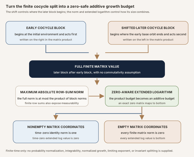
The picture separates three structures that are often conflated:
- the base map decides where the later cocycle block begins;
- matrix multiplication decides how the blocks compose; and
- the norm and logarithm decide how to summarize the size of that composition.
Each layer has its own assumptions and its own failure modes.
Base camp: the checked cocycle input
The preceding random-matrix-theory milestone 13 (RMT-13) fixes a type
\(\Omega\) of base states with a measurable-space structure, a finite matrix
index type \(\iota\) with decidable equality, and a measure \(\mu\) on
\(\Omega\). A bundled DiscreteMatrixCocycle μ stores:
- a base map \(T:\Omega\to\Omega\);
- a complex matrix generator \(A:\Omega\to M_\iota(\mathbb C)\);
- evidence that \(T\) preserves \(\mu\); and
- ordinary measurability of \(A\).
The measure-preserving field gives ordinary measurability of \(T\). RMT-13 therefore proves that every finite value
\[ \omega\longmapsto C(k,\omega) \]is measurable.
Random-matrix-theory milestone 14 (RMT-14), the target of this chapter, consumes exactly that interface. It does not add a probability instance for \(\mu\), and none of its finite-time pointwise inequalities uses measure preservation. The stored measurable structure matters for the two observable measurability theorems; the algebraic inequalities follow pointwise from the cocycle law and matrix norm.
That separation is useful. A theorem about one fixed \(\omega\) should not quietly depend on probability or ergodicity.
Camp one: why this particular matrix norm
For a finite complex matrix \(B=(B_{ij})\), define
\[ \lVert B\rVert_\infty {} = \max_{i\in\iota}\sum_{j\in\iota}|B_{ij}|. \]For each row, add the absolute values of all entries. Then keep the largest row total. This is the maximum absolute row-sum norm.
Why does it control column-vector evolution? Give \(x=(x_j)\) the supremum norm
\[ \lVert x\rVert_\infty=\max_j|x_j|. \]For the \(i\)-th output coordinate,
\[ \begin{aligned} |(Bx)_i| &=\left|\sum_j B_{ij}x_j\right|\\ &\leq\sum_j|B_{ij}|\,|x_j|\\ &\leq\left(\sum_j|B_{ij}|\right)\lVert x\rVert_\infty. \end{aligned} \]Taking the maximum over \(i\) yields
\[ \lVert Bx\rVert_\infty \leq \lVert B\rVert_\infty\lVert x\rVert_\infty. \]Mathlib proves that the row-sum formula agrees with the operator norm of the associated continuous linear map between finite function spaces carrying the supremum norm (Mathlib contributors).
This norm is not the Frobenius norm
\[ \lVert B\rVert_F {} = \left(\sum_{i,j}|B_{ij}|^2\right)^{1/2}, \]and it is not the Euclidean spectral operator norm. It is chosen because Mathlib already gives it a submultiplicative normed-ring interface and because it naturally controls supremum-norm vector evolution.
The Lean scope is semantic
Finite matrices admit several useful norms. Mathlib therefore does not install one matrix norm globally as the only possible interpretation. The module opens
open scoped Matrix.Norms.Operator
before using ‖B‖. Under that scope, the notation means the maximum
absolute row-sum norm. The theorem
normObservable_eq_rowSumSup then exposes the precise finite formula
in the public interface.
Camp two: define the finite-time norm observable
The first declaration is
def normObservable
    (C : DiscreteMatrixCocycle (ι := ι) μ) (k : ℕ) : Ω → ℝ :=
  fun ω ↦ ‖C.value k ω‖
Write
\[ N_k(\omega)=\lVert C(k,\omega)\rVert_\infty. \]The result is a real-valued function on base states. It is nonnegative because it is a norm, but the definition does not package that fact into a nonnegative real codomain. The later logarithm deliberately takes the extended norm notation instead.
The second declaration states the exact formula
\[ N_k(\omega) {} = \max_{i\in\iota} \sum_{j\in\iota}|C(k,\omega)_{ij}|. \]In Lean, the maximum is a Finset.sup in the nonnegative real type,
and the final value is coerced to an ordinary real. This representation has a
defined empty-family supremum, which will matter at the dimension boundary.
Camp three: zero time, one step, and a split
The RMT-13 value equations immediately give two normalization identities.
At time one,
\[ N_1(\omega)=\lVert A(\omega)\rVert_\infty, \]because the one-step cocycle value is the generator. This theorem needs no positive-dimension assumption.
At time zero, the value is the identity matrix. In nonempty dimension,
\[ N_0(\omega)=\lVert I\rVert_\infty=1. \]This is normObservable_zero, and its
Nonempty ι hypothesis is essential. In empty dimension the row
maximum is taken over no rows and equals zero.
For a split into \(m\) early steps and \(k\) shifted later steps, substitute the cocycle law into the norm:
\[ \begin{aligned} N_{m+k}(\omega) &=\left\lVert C(k,T^m\omega)C(m,\omega)\right\rVert_\infty\\ &\leq \lVert C(k,T^m\omega)\rVert_\infty \lVert C(m,\omega)\rVert_\infty\\ &=N_k(T^m\omega)N_m(\omega). \end{aligned} \]The theorem normObservable_add_le is pointwise and needs no
Nonempty ι. Matrix norm submultiplicativity remains true on the
trivial empty matrix space.
The order of terms mirrors matrix action. The shifted later block appears first in the product on the right because it is the left matrix factor. Since real multiplication commutes, the numerical product would be unchanged if written in the other order, but keeping the cocycle order visible prevents the underlying noncommutative statement from being forgotten.
Camp four: prove norm measurability from entries
It is tempting to say “norms are continuous, so the norm observable is measurable.” That shortcut would skip a project-specific seam. The random matrix measurable space was introduced entrywise, while the matrix norm comes from a scoped analytic instance. RMT-14 proves the connection directly rather than silently assuming those structures coincide in the needed way.
Start with the RMT-13 theorem
\[ \omega\longmapsto C(k,\omega) \quad\text{is measurable.} \]The proof of measurable_normObservable then climbs four finite
closure steps.
Step one: extract a measurable entry
For fixed \(i,j\in\iota\),
\[ \omega\longmapsto C(k,\omega)_{ij} \]is measurable by RandomMatrix.measurable_entry.
Step two: take the complex norm
The map
\[ \omega\longmapsto |C(k,\omega)_{ij}| \]is measurable. The Lean proof uses the nonnegative norm method
.nnnorm, so the values lie in the nonnegative reals.
Step three: sum one row
For each fixed row \(i\), the finite sum
\[ \omega\longmapsto\sum_{j\in\iota}|C(k,\omega)_{ij}| \]is measurable by Finset.measurable_sum.
Step four: take the finite supremum over rows
The proof establishes measurability for the supremum over an arbitrary finite
set of rows by induction. The empty supremum is the constant zero function.
Inserting a row replaces the previous supremum by the maximum of two
measurable functions. The Measurable.max closure theorem finishes
that step.
Finally, Matrix.linfty_opNorm_def identifies this finite supremum
with the scoped matrix norm, and coercion from nonnegative reals to reals
preserves measurability.
This proof works in empty dimension because both finite induction base cases are explicit.
Camp five: why the ordinary real logarithm is the wrong totalization
For a positive real \(r\), the ordinary logarithm changes multiplication into addition:
\[ \log(rs)=\log r+\log s. \]The boundary \(r=0\) creates the design problem. Mathematically, one usually
thinks of \(\log r\) tending to negative infinity as \(r\) decreases to zero.
Lean’s Real.log is a total function on all real inputs and uses
That convention is useful for total theorem statements, but it is wrong for this observable. It would assign the same logarithmic value to norm zero and norm one:
\[ \operatorname{Real.log}(0)=0=\operatorname{Real.log}(1). \]Exact matrix collapse would look like neutral size.
The module instead uses two extended number systems.
Extended nonnegative real input
Mathlib’s type ℝ≥0∞, also named ENNReal, contains all
nonnegative real numbers together with a top endpoint. The extended norm
notation ‖B‖ₑ lands there.
Extended real output
Mathlib’s EReal contains the real line together with bottom and
top endpoints. The function
ENNReal.log : ℝ≥0∞ → EReal
satisfies
\[ \operatorname{ENNReal.log}(0)=\bot, \qquad \operatorname{ENNReal.log}(1)=0, \]is strictly increasing, and obeys an unconditional product-to-sum identity (Mathlib contributors).
The seventh public declaration is therefore
def logNormObservable
    (C : DiscreteMatrixCocycle (ι := ι) μ) (k : ℕ) : Ω → EReal :=
  fun ω ↦ ENNReal.log ‖C.value k ω‖ₑ
Write this value as \(L_k(\omega)\).
Camp six: bottom exactly characterizes collapse
The theorem logNormObservable_eq_bot_iff states
This is an exact pointwise equivalence, not merely one implication. It follows from the exact endpoint theorem
\[ \operatorname{ENNReal.log}(r)=\bot \quad\Longleftrightarrow\quad r=0 \]and the zero-norm criterion.
Bottom has a semantic role. It means the finite matrix value is exactly the zero matrix. It does not mean “unknown,” “not measurable,” “outside the domain,” or “the proof failed.”
When the matrix value is nonzero, its norm is positive and finite, so the extended log norm agrees with an ordinary finite real logarithm. The sign has a direct finite-time interpretation:
\[ \begin{array}{c|c} L_k(\omega)\lt0 & 0\lt N_k(\omega)\lt1\\ L_k(\omega)=0 & N_k(\omega)=1\\ L_k(\omega)\gt0 & N_k(\omega)\gt1. \end{array} \]These are worst-case operator-norm budgets. A negative value gives a strict supremum-norm contraction bound for the complete finite matrix, but a positive value does not force every vector to grow, and a zero value does not identify the matrix with the identity. A nonzero singular matrix still has a finite log-norm value; bottom characterizes the zero matrix, not singularity.
The one-step and time-zero identities follow the norm layer:
\[ L_1(\omega) {} = \operatorname{ENNReal.log}\lVert A(\omega)\rVert_{\infty,e}, \]and, when \(\iota\) is nonempty,
\[ L_0(\omega)=0. \]The subscript \(e\) in the first display only reminds us that the norm has been embedded into the extended nonnegative reals. It does not select a new matrix norm.
Measurability of the extended log norm
The theorem measurable_logNormObservable composes three checked
maps:
- the real-valued norm observable is measurable;
ENNReal.ofRealmeasurably embeds its nonnegative values; andENNReal.logis measurable.
The key Mathlib identity ofReal_norm reconciles the real norm
followed by ENNReal.ofReal with the extended norm notation used in
the definition.
Measurability reaches no further. It does not show that the extended value is integrable, that its positive or negative parts have finite integral, or that bottom occurs only on a null set.
Camp seven: the zero-safe subadditivity proof
The theorem logNormObservable_add_le states
Its proof is a compact four-link chain.
Link one: rewrite by the cocycle law
Replace the full matrix value with the shifted later block times the early block:
\[ C(m+k,\omega) {} = C(k,T^m\omega)C(m,\omega). \]Link two: apply the extended norm product bound
The chosen matrix norm is submultiplicative:
\[ \left\lVert C(k,T^m\omega)C(m,\omega)\right\rVert_{\infty,e} \leq \lVert C(k,T^m\omega)\rVert_{\infty,e} \lVert C(m,\omega)\rVert_{\infty,e}. \]The Lean proof starts with the nonnegative norm inequality
nnnorm_mul_le, then coerces it into ENNReal.
Link three: use logarithm monotonicity
Because ENNReal.log is monotone, the preceding norm inequality can
be passed through the logarithm without reversing its direction.
Link four: turn the product into a sum
Mathlib’s ENNReal.log_mul_add gives
for all extended nonnegative \(r\) and \(s\), including zero and top endpoints. For finite matrix norms only the finite and zero cases arise, but the theorem does not need to split them.
This makes the proof zero-safe. No assumption says that either block is invertible or nonzero.
Nonzero factors can still collapse
Even if both block matrices are nonzero, their product may be zero. For example,
\[ B= \begin{bmatrix} 1 & 0\\ 0 & 0 \end{bmatrix}, \qquad D= \begin{bmatrix} 0 & 0\\ 0 & 1 \end{bmatrix} \]are nonzero but \(DB=0\). Then the full log norm is bottom while both block log norms are zero, since both block norms equal one. The inequality reads
\[ \bot\leq0+0, \]which is true. This example also shows why subadditivity is an inequality, not an equality.
Return to the two sample paths after the general theorem
Split each horizon-two path after its first factor, so \(m=k=1\). On the positive path, the norm theorem reads
\[ 2=N_2(p_0) \leq N_1(p_1)N_1(p_0) =2\cdot2=4, \]and extended-log subadditivity reads
\[ \log2=L_2(p_0) \leq L_1(p_1)+L_1(p_0) =\log2+\log2. \]On the collapse path,
\[ 0=N_2(z_0)\leq1\cdot1, \]while both one-step extended logs are zero and the full extended log is bottom:
\[ \bot=L_2(z_0)\leq0+0. \]The positive-log successor instead reports \(G_2(z_0)=0\). The values satisfy their own theorems; they answer different questions.
Type the two ledgers yourself with Lean and Std
The project modules use Mathlib’s general matrices, measurable cocycles,
extended reals, and operator norm. A learner can first verify the exact integer
products, row-sum norms, and symbolic zero policies with a bounded file that
imports only Std.
Create a scratch directory outside formalization/. Save this exact
block as FiniteCocycleObservablesTutorial.lean:
import Std

namespace FiniteCocycleObservablesTutorial

structure Matrix2 where
  a00 : Int
  a01 : Int
  a10 : Int
  a11 : Int
  deriving Repr, DecidableEq

def Matrix2.mul (A B : Matrix2) : Matrix2 :=
  { a00 := A.a00 * B.a00 + A.a01 * B.a10
    a01 := A.a00 * B.a01 + A.a01 * B.a11
    a10 := A.a10 * B.a00 + A.a11 * B.a10
    a11 := A.a10 * B.a01 + A.a11 * B.a11 }

def Matrix2.linftyOpNorm (A : Matrix2) : Nat :=
  max (A.a00.natAbs + A.a01.natAbs)
      (A.a10.natAbs + A.a11.natAbs)

def A0 : Matrix2 :=
  { a00 := 1, a01 := 1, a10 := 0, a11 := 1 }

def A1 : Matrix2 :=
  { a00 := 1, a01 := 0, a10 := 0, a11 := 2 }

def B0 : Matrix2 :=
  { a00 := 1, a01 := 0, a10 := 0, a11 := 0 }

def B1 : Matrix2 :=
  { a00 := 0, a01 := 0, a10 := 0, a11 := 1 }

def positiveProduct : Matrix2 := A1.mul A0
def collapseProduct : Matrix2 := B1.mul B0

inductive LogValue where
  | bottom
  | zero
  | logOfNat (n : Nat)
  deriving Repr, DecidableEq

def positiveLogToken (n : Nat) : LogValue :=
  if n ≤ 1 then .zero else .logOfNat n

def extendedLogToken (n : Nat) : LogValue :=
  if n = 0 then .bottom
  else if n = 1 then .zero
  else .logOfNat n

structure FiniteQuotient where
  numerator : LogValue
  factorCount : Nat
  deriving Repr, DecidableEq

def normalizeAt (k : Nat) (value : LogValue) : Option FiniteQuotient :=
  if k = 0 then none else some { numerator := value, factorCount := k }

structure ObservableLedger where
  product : Matrix2
  productNorm : Nat
  factorNormBudget : Nat
  positiveLog : LogValue
  extendedLog : LogValue
  normalizedPositiveLog : Option FiniteQuotient
  normalizedExtendedLog : Option FiniteQuotient
  deriving Repr, DecidableEq

def ledger (left right : Matrix2) : ObservableLedger :=
  let product := left.mul right
  let norm := product.linftyOpNorm
  { product := product
    productNorm := norm
    factorNormBudget := left.linftyOpNorm * right.linftyOpNorm
    positiveLog := positiveLogToken norm
    extendedLog := extendedLogToken norm
    normalizedPositiveLog := normalizeAt 2 (positiveLogToken norm)
    normalizedExtendedLog := normalizeAt 2 (extendedLogToken norm) }

def positiveLedger : ObservableLedger := ledger A1 A0
def collapseLedger : ObservableLedger := ledger B1 B0

#eval [positiveProduct, collapseProduct]
#eval [A0.linftyOpNorm, A1.linftyOpNorm,
  positiveProduct.linftyOpNorm,
  B0.linftyOpNorm, B1.linftyOpNorm,
  collapseProduct.linftyOpNorm]
#eval positiveLedger
#eval collapseLedger
#eval [positiveLogToken 0, positiveLogToken 1, positiveLogToken 2]
#eval [extendedLogToken 0, extendedLogToken 1, extendedLogToken 2]
#eval normalizeAt 0 (.logOfNat 2)

example : positiveProduct =
    { a00 := 1, a01 := 1, a10 := 0, a11 := 2 } := by decide
example : collapseProduct =
    { a00 := 0, a01 := 0, a10 := 0, a11 := 0 } := by decide
example : positiveProduct.linftyOpNorm = 2 := by decide
example : collapseProduct.linftyOpNorm = 0 := by decide
example : positiveLedger.factorNormBudget = 4 := by decide
example : collapseLedger.factorNormBudget = 1 := by decide
example : positiveLedger.positiveLog = .logOfNat 2 := by decide
example : positiveLedger.extendedLog = .logOfNat 2 := by decide
example : collapseLedger.positiveLog = .zero := by decide
example : collapseLedger.extendedLog = .bottom := by decide
example : normalizeAt 0 (.logOfNat 2) = none := by decide

end FiniteCocycleObservablesTutorial
Open a terminal in that scratch directory and type:
source "$HOME/.elan/env"
elan run leanprover/lean4:v4.32.0 lean FiniteCocycleObservablesTutorial.lean
Resource label: small standalone Lean tutorial, ordinary Mac or Linux. This exact worksheet was executed with Lean 4.32.0 and printed:
[{ a00 := 1, a01 := 1, a10 := 0, a11 := 2 }, { a00 := 0, a01 := 0, a10 := 0, a11 := 0 }]
[2, 2, 2, 1, 1, 0]
{ product := { a00 := 1, a01 := 1, a10 := 0, a11 := 2 },
  productNorm := 2,
  factorNormBudget := 4,
  positiveLog := FiniteCocycleObservablesTutorial.LogValue.logOfNat 2,
  extendedLog := FiniteCocycleObservablesTutorial.LogValue.logOfNat 2,
  normalizedPositiveLog := some { numerator := FiniteCocycleObservablesTutorial.LogValue.logOfNat 2, factorCount := 2 },
  normalizedExtendedLog := some { numerator := FiniteCocycleObservablesTutorial.LogValue.logOfNat 2,
                             factorCount := 2 } }
{ product := { a00 := 0, a01 := 0, a10 := 0, a11 := 0 },
  productNorm := 0,
  factorNormBudget := 1,
  positiveLog := FiniteCocycleObservablesTutorial.LogValue.zero,
  extendedLog := FiniteCocycleObservablesTutorial.LogValue.bottom,
  normalizedPositiveLog := some { numerator := FiniteCocycleObservablesTutorial.LogValue.zero, factorCount := 2 },
  normalizedExtendedLog := some { numerator := FiniteCocycleObservablesTutorial.LogValue.bottom, factorCount := 2 } }
[FiniteCocycleObservablesTutorial.LogValue.zero,
 FiniteCocycleObservablesTutorial.LogValue.zero,
 FiniteCocycleObservablesTutorial.LogValue.logOfNat 2]
[FiniteCocycleObservablesTutorial.LogValue.bottom,
 FiniteCocycleObservablesTutorial.LogValue.zero,
 FiniteCocycleObservablesTutorial.LogValue.logOfNat 2]
none
Read the output in layers:
- the two products are the positive matrix and the zero matrix;
- the factor and product norms are \(2,2,2\) and \(1,1,0\);
- the positive ledger stores the symbolic numerator \(\log2\) in both logarithm slots and the factor count two;
- the collapse ledger stores zero for the positive logarithm and bottom for the extended logarithm;
- the separate token lists expose the policies at norms zero, one, and two; and
- conventional normalization at horizon zero returns
none.
LogValue.logOfNat 2 is a symbolic token for the exact expression
\(\log2\); the worksheet does not approximate a transcendental number.
Likewise, LogValue.bottom models the zero policy without
reimplementing Mathlib’s EReal. Every integer product, norm,
budget, branch, and example is kernel-checked. The project-level
types and theorems remain the full project interfaces in the earlier
repository checks.
The worksheet’s normalizeAt 0 = none intentionally models the
classical partial convention that normalization needs a positive horizon. It
is not an implementation of the much later real
normalizedProcess, whose explicitly totalized time-zero value is
zero.
Camp eight: positive and empty dimensions
The module treats the matrix index type \(\iota\) as finite, but does not assume it is inhabited unless a theorem needs the familiar identity normalization.
Nonempty coordinate type
If \(\iota\) has at least one index, the identity matrix has one in every diagonal position and zero elsewhere. Every row has absolute sum one, so
\[ \lVert I\rVert_\infty=1. \]Therefore
\[ N_0(\omega)=1, \qquad L_0(\omega)=0. \]Only normObservable_zero and
logNormObservable_zero add Nonempty ι to the module’s
finite-index assumptions.
Empty coordinate type
If \(\iota\) is empty, there are no matrix entries. There is exactly one square matrix function, so the zero and identity matrices are equal. The maximum absolute row-sum formula takes the supremum of an empty family and returns zero. Thus, at every horizon and base state,
\[ N_k(\omega)=0, \qquad L_k(\omega)=\bot. \]The final two public theorems state those functions exactly:
normObservable_eq_zero_of_isEmpty; andlogNormObservable_eq_bot_of_isEmpty.
The second theorem reuses the exact bottom criterion after proving that the unique empty matrix equals zero.
There is no contradiction between “time-zero value is the identity” and “time-zero log norm is bottom” in empty dimension. The unique identity is also the zero matrix, and its empty row-sum norm is zero.
The complete fourteen-declaration map
All declarations share a measurable base space \(\Omega\), a finite matrix
index type \(\iota\) with decidable equality, an arbitrary measure \(\mu\), and a
bundled complex DiscreteMatrixCocycle. The table lists every
additional assumption and exact result.
| # | Declaration | Additional assumption | Checked content |
|---|---|---|---|
| 1 | normObservable | None | Defines the real maximum-row-sum norm of the finite cocycle value |
| 2 | normObservable_eq_rowSumSup | None | Exposes the exact finite supremum of absolute row sums |
| 3 | normObservable_zero | Nonempty ι | Time-zero norm observable is the constant one function |
| 4 | normObservable_one | None | One-step norm is the generator norm |
| 5 | normObservable_add_le | None | Full norm is bounded by shifted later-block norm times early-block norm |
| 6 | measurable_normObservable | None | Every finite norm observable is ordinarily measurable |
| 7 | logNormObservable | None | Defines the EReal-valued extended logarithm of the extended norm |
| 8 | logNormObservable_eq_bot_iff | None | Extended log norm is bottom exactly when the finite matrix value is zero |
| 9 | logNormObservable_zero | Nonempty ι | Time-zero extended log norm is the constant zero function |
| 10 | logNormObservable_one | None | One-step value is the extended log norm of the generator |
| 11 | measurable_logNormObservable | None | Every finite extended log-norm observable is measurable |
| 12 | logNormObservable_add_le | None | Extended log norms are subadditive across every shifted cocycle split |
| 13 | normObservable_eq_zero_of_isEmpty | IsEmpty ι | Every finite norm observable is the constant zero function |
| 14 | logNormObservable_eq_bot_of_isEmpty | IsEmpty ι | Every finite log-norm observable is the constant bottom function |
The declaration order is deliberate. The row-sum formula comes before the measurability proof that consumes it. The exact bottom criterion comes before the empty-dimension log theorem that reuses it.
The proof architecture
The module is short because each theorem consumes a precise upstream law.
Norm layer
C.value_zeroand Mathlib’s norm-one instance prove time zero in nonempty dimension.C.value_oneproves the one-step generator identity.C.value_addplusnorm_mul_leproves the split bound.C.measurable_value, measurable entries, finite sums, finite maxima, andMatrix.linfty_opNorm_defprove measurability.
Extended-log layer
ENNReal.log_eq_bot_iffand norm zero equivalence prove the exact collapse criterion.ENNReal.log_oneproves the positive-dimensional zero-time law.C.value_oneproves the generator identity.- measurable embedding plus
Measurable.ennreal_logproves measurability. - cocycle splitting,
nnnorm_mul_le, logarithm monotonicity, andENNReal.log_mul_addprove subadditivity.
Empty-dimension layer
Function extensionality and empty elimination show that every matrix value is the zero matrix. The norm theorem then simplifies directly, and the log theorem uses the exact bottom criterion.
No proof needs a matrix inverse, determinant, eigenvalue, singular value, probability instance, integral, or limit.
Assumption and type ledger
| Object | Type | What is known | What is not inferred |
|---|---|---|---|
| Base measure | Measure Ω | The cocycle base preserves it | Total mass one, ergodicity, or finiteness |
| Finite cocycle value | Ω → Matrix ι ι ℂ | Measurable, with zero/one/add laws | Invertibility, a law, or integrability |
| Norm observable | Ω → ℝ | Measurable and submultiplicative across splits | Expectation, lower bound, or normalized limit |
| Extended norm | ℝ≥0∞ pointwise | Exact coercion of the finite norm | A new matrix norm or an infinite finite-matrix value |
| Extended log norm | Ω → EReal | Measurable, bottom exactly at zero, subadditive | Integrability, almost-sure finiteness, or Lyapunov exponent |
The word “observable” means a measurable function of the base state at a fixed horizon. It does not mean a physical measurement postulate or an expectation.
Why this layer matters
Matrix cocycle growth is the bridge between several future tracks:
- derivatives of nonlinear iterates can form matrix cocycles after a checked chain-rule construction;
- products of random matrices become cocycles when driven by a common base dynamics;
- finite norm bounds are raw material for stability and contraction criteria; and
- integrable log norms are among the hypotheses used in multiplicative ergodic theory.
But a bridge must begin with exact endpoints. Defining a real logarithm at zero without care would corrupt every later statement about collapse or asymptotic growth. Hiding the matrix norm would make constants and geometry ambiguous. Assuming measurability without connecting it to the project-owned matrix structure would leave a formal gap.
RMT-14 closes those finite-time seams and stops.
Common wrong turns
Calling the selected norm Frobenius
The active norm is the largest absolute row sum. Frobenius geometry sums the squares of every entry and then takes a square root. Those norms are not equal and support different proof interfaces.
Assuming norm notation is globally unambiguous
The meaning of ‖B‖ depends on
open scoped Matrix.Norms.Operator. The explicit row-sum theorem is
the audit trail.
Declaring measurability by continuity alone
The project’s matrix measurable structure is entrywise. The module proves measurability from measurable entries, finite sums, and finite suprema before using the row-sum identity.
Applying Real.log to the norm
Its total value at zero is zero, which would confuse exact collapse with norm
one. The checked observable uses ENNReal.log into
EReal.
Treating bottom as an error
Bottom is the exact intended value if and only if the cocycle matrix is zero. It is part of the mathematical codomain.
Assuming nonzero blocks have a nonzero product
Matrices can be zero divisors. The extended-real inequality remains valid when the full product collapses even though neither block is zero.
Replacing subadditivity with equality
The logarithm turns a product of norm bounds into a sum, but the matrix norm is only submultiplicative. Slack or complete collapse can occur.
Adding an unnecessary nonempty-dimension assumption
Only the familiar time-zero normalizations need an inhabited coordinate type. Definitions, measurability, inequalities, and explicit empty-dimension laws do not.
Reading measurability as integrability
A measurable extended-real function can fail every integrability condition needed later. The module evaluates no integral.
Reading subadditivity as Kingman’s theorem
A finite pointwise inequality is one input to subadditive ergodic theory. It is not a probability space, an integrability theorem, an ergodicity theorem, or a limit.
Reading a log-norm observable as a Lyapunov exponent
A Lyapunov exponent is asymptotic growth after a normalization and under additional hypotheses. \(L_k(\omega)\) is a finite-horizon value.
Assuming a nonlinear Jacobian origin
The generator is an arbitrary measurable complex matrix map. No nonlinear map, derivative, chain rule, or tangent-space identification appears here.
Exercises from trailhead to summit
Trailhead
- Compute the largest absolute row sum of three different two-by-two matrices.
- Verify both running horizon-two products entry by entry.
- Give a nonidentity matrix with maximum absolute row-sum norm one.
- Explain in words why one output coordinate corresponds to one matrix row.
- Compare the row-sum norm and Frobenius norm of the identity in dimensions one, two, and three.
- Build the four-row norm, positive-log, and extended-log table without looking back at the figure.
Mid-mountain
- Derive matrix-vector control from the triangle inequality.
- Derive the cocycle norm split from
C.value_addandnorm_mul_le. - Reconstruct the measurable-row-sum proof for a two-row matrix.
- Generalize that proof by induction over an arbitrary finite set of rows.
- Track the types in the composition from a real norm through
ENNReal.ofRealtoENNReal.log. - Prove on paper that bottom characterizes a zero matrix.
- Find two nonzero matrices with zero product and evaluate both sides of the extended log-norm inequality.
- Explain why the norm split and log split need no probability assumption.
Summit
- Audit every theorem in the fourteen-declaration map against its exact assumptions.
- Prove that the empty square matrix is simultaneously zero and identity.
- Derive the constant-zero norm and constant-bottom log-norm functions in empty dimension.
- State a candidate integrability hypothesis for the one-step positive log norm and explain why it is absent here.
- Compare finite subadditivity with the hypotheses and conclusion of Kingman’s subadditive ergodic theorem.
- State the additional probability, invertibility, and integrability choices needed before an Oseledets theorem could even be formulated.
- Design a separate theorem connecting the cocycle generator to a Jacobian along a nonlinear orbit. List the differentiability and chain-rule prerequisites.
- Normalize both running logarithm ledgers at horizon two, then explain why the target module proves neither a normalized-process theorem nor a limit.
Reproduce the chapter
The bounded Std worksheet above is a standalone tutorial for an
ordinary macOS or Linux host. The exact target and comparison modules import
Mathlib and are full project checks. From the repository root, run:
cd formalization
lake env lean NonlinearDynamics/Random/RandomCocycles/NormObservables.lean
lake env lean NonlinearDynamics/Random/RandomCocycles/LogPlusIntegrability.lean
lake env lean NonlinearDynamics/Random/RandomCocycles/SubadditiveKingman.lean
These commands may require substantial disk space and memory. Passing the technical gates would still leave human mathematical, source, accessibility, scientific-integrity, and editorial review pending.
Summit: what has and has not been proved
| Topic | Status in this module |
|---|---|
| Finite-time maximum absolute row-sum norm observable | Defined |
| Exact finite row-sum supremum formula | Checked |
| Positive-dimensional time-zero norm one | Checked under Nonempty ι |
| One-step generator norm identity | Checked |
| Norm submultiplicativity across the shifted cocycle split | Checked pointwise |
| Entrywise proof of norm measurability | Checked |
| Extended-real log-norm observable | Defined through ENNReal.log |
| Exact bottom if and only if zero-matrix criterion | Checked |
| Positive-dimensional time-zero log value zero | Checked under Nonempty ι |
| One-step generator extended-log-norm identity | Checked |
| Extended log-norm measurability | Checked |
| Extended-real subadditivity across every cocycle split | Checked pointwise |
| Empty-dimensional norm identically zero | Checked under IsEmpty ι |
| Empty-dimensional log norm identically bottom | Checked under IsEmpty ι |
| Real log-positive envelope \(G_k\) | Defined only in the successor LogPlusIntegrability.lean |
| Integrability of finite \(G_k\) | Proved there only from an explicit one-step hypothesis |
| Positive-time quotients displayed in this chapter | Computed for the examples; not defined by the target module |
Generic real normalizedProcess | Defined much later; not an EReal normalizer |
| Extended log norm is everywhere an ordinary real value | Not proved and false when a finite value is zero |
| Probability normalization of the base measure | Not assumed or proved |
| Ergodicity, mixing, stationarity, or independence | Not assumed or proved |
| Integrability of the norm observable | Not proved |
| Integrability or almost-sure finiteness of the extended log norm | Not proved |
| Pushforward law or expectation of either observable | Not defined |
| Continuity in the base state, moment bounds, or tail estimates | Not proved |
| Skew-product invariance or product-law factorization | Not stated |
| Target-module normalized finite-time growth | Not defined |
| Subadditive ergodic limit | Not invoked or proved |
| Lyapunov exponent or spectrum | Not defined or proved |
| Oseledets invariant splitting | Not invoked or proved |
| Invertibility or negative-time cocycle | Not assumed or defined |
| General-linear-valued generator or two-sided group cocycle | Not assumed or defined |
| Singular-value, determinant, or spectral-radius formula | Not stated |
| Norm multiplicativity, log additivity, equality, or lower product-growth bound | Not stated |
| Comparison with Frobenius or Euclidean spectral norms | Not formalized |
| Matrix logarithm or the distinct ordinary-differential-equation logarithmic norm | Not defined |
| Nonlinear derivative or random-Jacobian representation | Not connected |
| Stability, attraction, bifurcation, or chaos theorem | Not claimed |
The summit is an analytic interface, not an asymptotic theorem. Every finite cocycle value now has a checked measurable size, every exact collapse remains visible as bottom, and every time split obeys a zero-safe additive upper bound.
Where to continue
Finite-Horizon Log-Positive Cocycle Integrability is the immediate successor. It defines the real nonnegative log-positive integrability envelope , majorizes every finite horizon by shifted one-step terms, and propagates an explicit generator integrability assumption through that finite sum. It does not make this chapter’s contraction-sensitive extended log norm integrable and does not prove a Lyapunov exponent.
The extended log-norm observable glossary entry is the compact guide to the type ladder, bottom convention, and dimension boundary.
Generator-Presented One-Sided Discrete Matrix Cocycles develops the exact base-orbit and later-block-left algebra consumed here. Ordered Finite Matrix Products and Operator-Norm Growth develops the deterministic product and maximum-row-sum norm layer below the cocycle.
The next asymptotic layer must state an integrability policy before normalizing by time or invoking a subadditive or multiplicative ergodic theorem. It must also decide whether the base measure is probabilistic and whether ergodicity, invertibility, or one-sided time is required. None of those choices is made retroactively here.
References
Mathlib contributors. Norms on finite matrices, Mathlib 4 documentation. This official source defines the maximum absolute row-sum norm, proves its matrix-product and matrix-vector bounds, and identifies it with the operator norm on finite supremum-norm function spaces.
Mathlib contributors.
Extended nonnegative-real logarithm,
Mathlib 4 documentation. This official source defines ENNReal.log,
including its zero-to-bottom convention, strict monotonicity, exact endpoint
criteria, and unconditional product-to-sum law.
Mathlib contributors. Extended logarithm and exponential, Mathlib 4 documentation. This official source packages the logarithm as an order isomorphism and homeomorphism and proves that it is measurable.
Mathlib contributors.
Positive part of the real logarithm,
Mathlib 4 documentation. This official source defines
Real.posLog as the maximum of zero and the real logarithm, proves
its zero policy, nonnegativity, continuity, and product upper bound.
Mathlib contributors. Extended-real inversion and division, Mathlib 4 documentation. This official source records that bottom divided by a positive finite extended real remains bottom. The target module itself defines no normalized extended observable.
Roger A. Horn and Charles R. Johnson. Matrix Analysis, second edition, Cambridge University Press, 2013, International Standard Book Number (ISBN) 978-0-521-54823-6. Chapter 5 develops vector norms, induced matrix norms, and submultiplicative product estimates.
J. F. C. Kingman. The ergodic theory of subadditive stochastic processes, Journal of the Royal Statistical Society, Series B 30(3), 1968, 499-510. This primary source establishes a subadditive ergodic theorem under additional measure-theoretic hypotheses. RMT-14 supplies only the finite pointwise subadditivity input.
V. I. Oseledets. A multiplicative ergodic theorem. Characteristic Ljapunov exponents of dynamical systems, Transactions of the Moscow Mathematical Society 19 (1968), 197-231. This primary source supplies the historical long-time destination. The present module proves none of its integrability, limit, exponent, or splitting conclusions.
Ludwig Arnold. Random Dynamical Systems, Springer Monographs in Mathematics, 1998. This develops cocycles and multiplicative ergodic theory over metric dynamical systems. Its usual probability, invertibility, and asymptotic structures are context, not claims of this finite-time module.
The exact upstream Lean source audited for this chapter is Mathlib commit
81a5d257,
the revision pinned by formalization/lake-manifest.json.