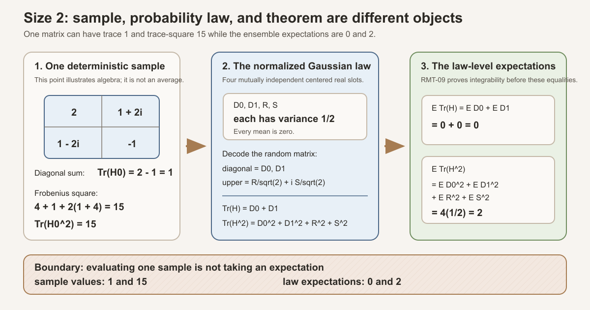
Start with one matrix, then change levels
The Gaussian unitary ensemble (GUE) is a probability law on finite Hermitian matrices . A probability law is an assignment of mass to measurable subsets of matrix space. It is not one matrix, and an expectation is a probability-weighted average under that law.
Those distinctions matter immediately. Begin with the deterministic matrix
\[ H_0= \begin{bmatrix} 2 & 1+2i\\ 1-2i & -1 \end{bmatrix}. \]Its ordinary, unnormalized matrix trace is
\[ \operatorname{Tr}(H_0)=2+(-1)=1. \]Hermiticity makes the trace of its square equal its Frobenius squared norm:
\[ \begin{aligned} \operatorname{Tr}(H_0^2) &=2^2+(-1)^2+2|1+2i|^2\\ &=4+1+2(1+4)\\ &=15. \end{aligned} \]The pair \((1,15)\) describes one point. It does not say what the GUE expectations are.
Put the size-two GUE law on normalized coordinates
For the repository’s size-two normalization, choose four mutually independent centered real Gaussian coordinates
\[ D_0,D_1,R,S\sim N(0,1/2). \]Here \(N(m,v)\) denotes a real Gaussian law with mean \(m\) and variance \(v\). “Centered” means mean zero. Mutual independence means the joint law is the product of all four scalar laws, not merely that each pair has zero covariance.
Decode those normalized coordinates as
\[ H= \begin{bmatrix} D_0 & R/\sqrt2+iS/\sqrt2\\ R/\sqrt2-iS/\sqrt2 & D_1 \end{bmatrix}. \]The displayed real and imaginary parts above the diagonal each have variance \((1/2)/2=1/4\). The normalized variables \(R,S\) themselves still have variance \(1/2\).
Now compute the two random observables pointwise:
\[ \operatorname{Tr}(H)=D_0+D_1, \]and
\[ \begin{aligned} \operatorname{Tr}(H^2) &=D_0^2+D_1^2 +2\left|R/\sqrt2+iS/\sqrt2\right|^2\\ &=D_0^2+D_1^2+R^2+S^2. \end{aligned} \]Each coordinate is centered, so linearity of expectation gives
\[ \mathbb E\operatorname{Tr}(H)=0+0=0. \]For a centered real Gaussian, the second moment equals the variance. Therefore
\[ \begin{aligned} \mathbb E\operatorname{Tr}(H^2) &=\mathbb E D_0^2+\mathbb E D_1^2 +\mathbb E R^2+\mathbb E S^2\\ &=\frac12+\frac12+\frac12+\frac12\\ &=2. \end{aligned} \]This last sum needs linearity, not a factorization of products of distinct coordinates. The product law is still essential because it is the exact source law from which the matrix law is pushed forward.
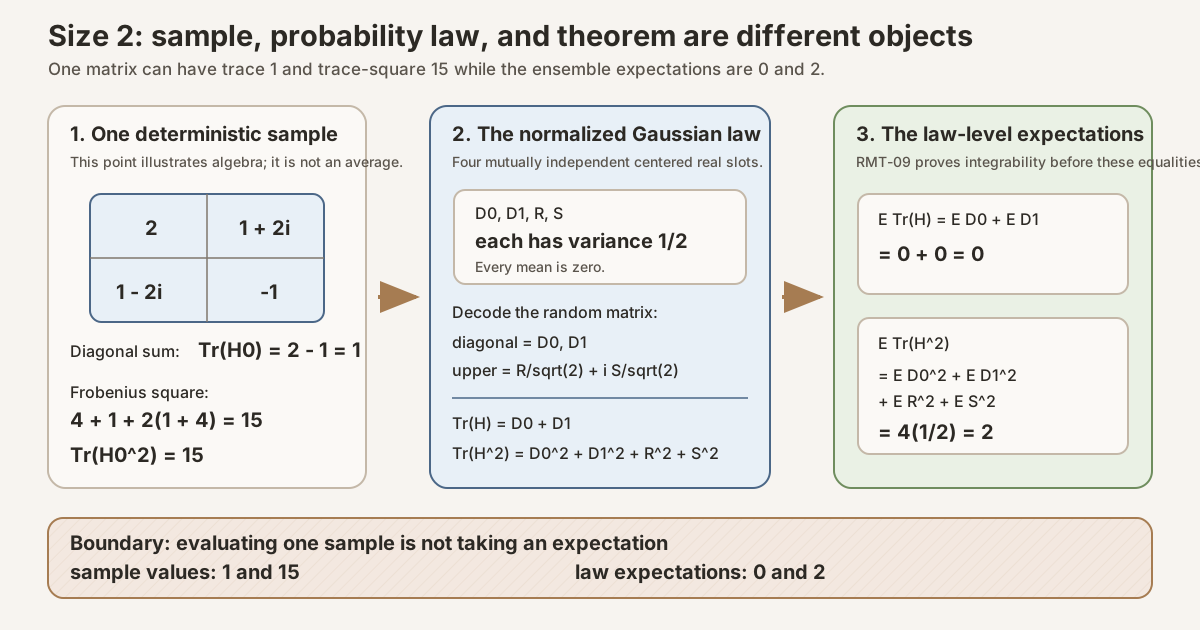
Three near-misses with three different answers
The correct value \(2\) depends on keeping the law, observable, and operation fixed.
- Wrong decoder. If the upper entry were \(R+iS\), without division by \(\sqrt2\), then \[ \mathbb E[D_0^2+D_1^2+2R^2+2S^2]=3. \] That is a different matrix law with the wrong Frobenius normalization.
- Wrong observable. The scalar square \((\operatorname{Tr}H)^2\) is not \(\operatorname{Tr}(H^2)\). Under the product law, \[ \mathbb E[(\operatorname{Tr}H)^2] =\mathbb E[(D_0+D_1)^2]=1. \] Off-diagonal energy never appears in this observable.
- Wrong probability level. Substitution of \(H_0\) produces \(15\), but no law has been integrated. A sample value is not an expected value.
Type and run the finite ledger yourself
The exact GUE measures and Bochner integrals are full project checks that
use Mathlib and may require substantial disk space and memory. The
deterministic matrix arithmetic and quarter-unit moment ledger form a
standalone tutorial that imports only Std.
Create /tmp/GUETraceMoments2Tutorial.lean and type:
import Std

structure ComplexInt where
  re : Int
  im : Int
deriving Repr, DecidableEq

def ComplexInt.add (z w : ComplexInt) : ComplexInt :=
  ⟨z.re + w.re, z.im + w.im⟩

def ComplexInt.mul (z w : ComplexInt) : ComplexInt :=
  ⟨z.re * w.re - z.im * w.im,
    z.re * w.im + z.im * w.re⟩

structure Matrix2 where
  a00 : ComplexInt
  a01 : ComplexInt
  a10 : ComplexInt
  a11 : ComplexInt
deriving Repr, DecidableEq

def Matrix2.entries (H : Matrix2) : List (Int × Int) :=
  [(H.a00.re, H.a00.im), (H.a01.re, H.a01.im),
   (H.a10.re, H.a10.im), (H.a11.re, H.a11.im)]

def Matrix2.trace (H : Matrix2) : ComplexInt :=
  H.a00.add H.a11

def Matrix2.traceSquare (H : Matrix2) : ComplexInt :=
  let diagonal0 := H.a00.mul H.a00
  let upperLower := H.a01.mul H.a10
  let lowerUpper := H.a10.mul H.a01
  let diagonal1 := H.a11.mul H.a11
  (diagonal0.add upperLower).add (lowerUpper.add diagonal1)

def sampleH : Matrix2 :=
  ⟨⟨2, 0⟩, ⟨1, 2⟩, ⟨1, -2⟩, ⟨-1, 0⟩⟩

def normalizedVarianceQuarters : List (String × Nat) :=
  [("diagonal 0", 2), ("diagonal 1", 2),
   ("upper real normalized", 2), ("upper imaginary normalized", 2)]

def diagonalMeans : List Int := [0, 0]

def expectedTrace : Int := diagonalMeans.sum

def expectedTraceSquareQuarters : Nat :=
  (normalizedVarianceQuarters.map Prod.snd).sum

def expectedSquareOfTraceQuarters : Nat :=
  2 + 2

def wrongDecoderTraceSquareQuarters : Nat :=
  2 + 2 + 2 * 2 + 2 * 2

def quarters (q : Nat) : Rat :=
  (q : Rat) / 4

#eval normalizedVarianceQuarters
#eval sampleH.entries
#eval sampleH.trace
#eval sampleH.traceSquare
#eval (expectedTrace, quarters expectedTraceSquareQuarters,
  quarters expectedSquareOfTraceQuarters,
  quarters wrongDecoderTraceSquareQuarters)
#eval (decide (sampleH.trace.re ≠ expectedTrace),
  decide (sampleH.traceSquare.re ≠ 2),
  decide (expectedTraceSquareQuarters ≠ wrongDecoderTraceSquareQuarters))

example : sampleH.trace = ⟨1, 0⟩ := by
  native_decide

example : sampleH.traceSquare = ⟨15, 0⟩ := by
  native_decide

example : expectedTrace = 0 := by
  native_decide

example : quarters expectedTraceSquareQuarters = 2 := by
  native_decide

example : quarters expectedSquareOfTraceQuarters = 1 := by
  native_decide

example : quarters wrongDecoderTraceSquareQuarters = 3 := by
  native_decide

example : sampleH.trace.re ≠ expectedTrace := by
  native_decide

example : sampleH.traceSquare.re ≠ 2 := by
  native_decide

example : expectedTraceSquareQuarters ≠
    wrongDecoderTraceSquareQuarters := by
  native_decide
Run the pinned compiler directly:
source "$HOME/.elan/env"
elan run leanprover/lean4:v4.32.0 lean /tmp/GUETraceMoments2Tutorial.lean
Resource label: small standalone Lean plus Std, suitable for an
ordinary macOS or Linux machine. This command does not enter the Lake
project, import Mathlib, or compile the formalization.
The executed output is:
[("diagonal 0", 2), ("diagonal 1", 2), ("upper real normalized", 2), ("upper imaginary normalized", 2)]
[(2, 0), (1, 2), (1, -2), (-1, 0)]
{ re := 1, im := 0 }
{ re := 15, im := 0 }
(0, 2, 1, 3)
(true, true, true)
The value 2 in every variance row means two quarter-units, or
\(1/2\). The tuple (0, 2, 1, 3) records expected trace, correct
expected matrix-square trace, expected squared scalar trace, and the
wrong-decoder result. Nine example declarations state the same
integer and rational identities as propositions checked by Lean’s kernel.
This worksheet does not construct a Gaussian random variable, prove integrability, or evaluate a Bochner integral. It checks the finite arithmetic that the exact Mathlib-backed theorems organize.
What RMT-09 proves in every finite dimension
The ninth random-matrix-theory milestone (RMT-09) crosses the analytic boundary. For every \(n\in\mathbb N\), including \(n=0\), it proves that the first two trace-power observables are complex Bochner integrable under the Wigner-scaled GUE matrix law and then evaluates their integrals:
\[ \mathbb E[\operatorname{Tr}(H)]=0, \qquad \mathbb E[\operatorname{Tr}(H^2)]=n. \]The theorem statements live in \(\mathbb C\) because the ambient matrices and trace observable are complex-valued, even though these values are real on Hermitian matrices. The checked module exposes exactly four public declarations: two integrability theorems and the two integral identities they license. It invokes no density, eigenvalue enumeration, or large-dimension limit.
Choose a route up
| Route | Begin with | Destination |
|---|---|---|
| First encounter | Two proofs in one picture | See why the powers use different structures |
| Analysis route | Why integrability is not bookkeeping | Understand the Bochner gate |
| Linear route | The first trace reads the diagonal | Derive the centered first moment |
| Geometry route | Hermitian trace square is Frobenius energy | Convert the second trace power into a norm square |
| Probability route | Move the law to normalized real coordinates | Reduce the second moment to scalar Gaussian squares |
| Arithmetic route | Count the coordinates and close the normalization | Explain the exact dimension factor and zero branch |
| Lean route | The four checked declarations | Audit the final public API and proof architecture |
| Boundary route | What has and has not been proved | Separate finite identities from spectral context |
Learning objectives
By the summit, you should be able to:
- distinguish a trace-power observable from its expected trace moment;
- state Bochner integrability for a complex-valued function;
- explain why Mathlib’s total integral makes a separate integrability theorem mathematically important;
- move an integral and an integrability claim through a measurable pushforward without conflating the two;
- derive the first expected trace from centered diagonal Gaussian marginals;
- prove pointwise that the trace square of a Hermitian matrix is its Frobenius norm square;
- translate that norm square into a sum of normalized real coordinate squares;
- use a scalar centered Gaussian second moment to integrate the finite sum;
- explain why linearity, not independence, closes the second calculation;
- count the normalized coordinates using the finite index equivalence with all matrix positions;
- reconcile the positive-dimensional division by \(n\) with the separate zero-dimensional branch;
- audit the Wigner normalization from displayed entry variances through the final trace identity;
- state all four Lean theorems with their exact codomains and measures; and
- separate the checked finite identities from density, eigenvalue, and asymptotic statements.
Two proofs in one picture
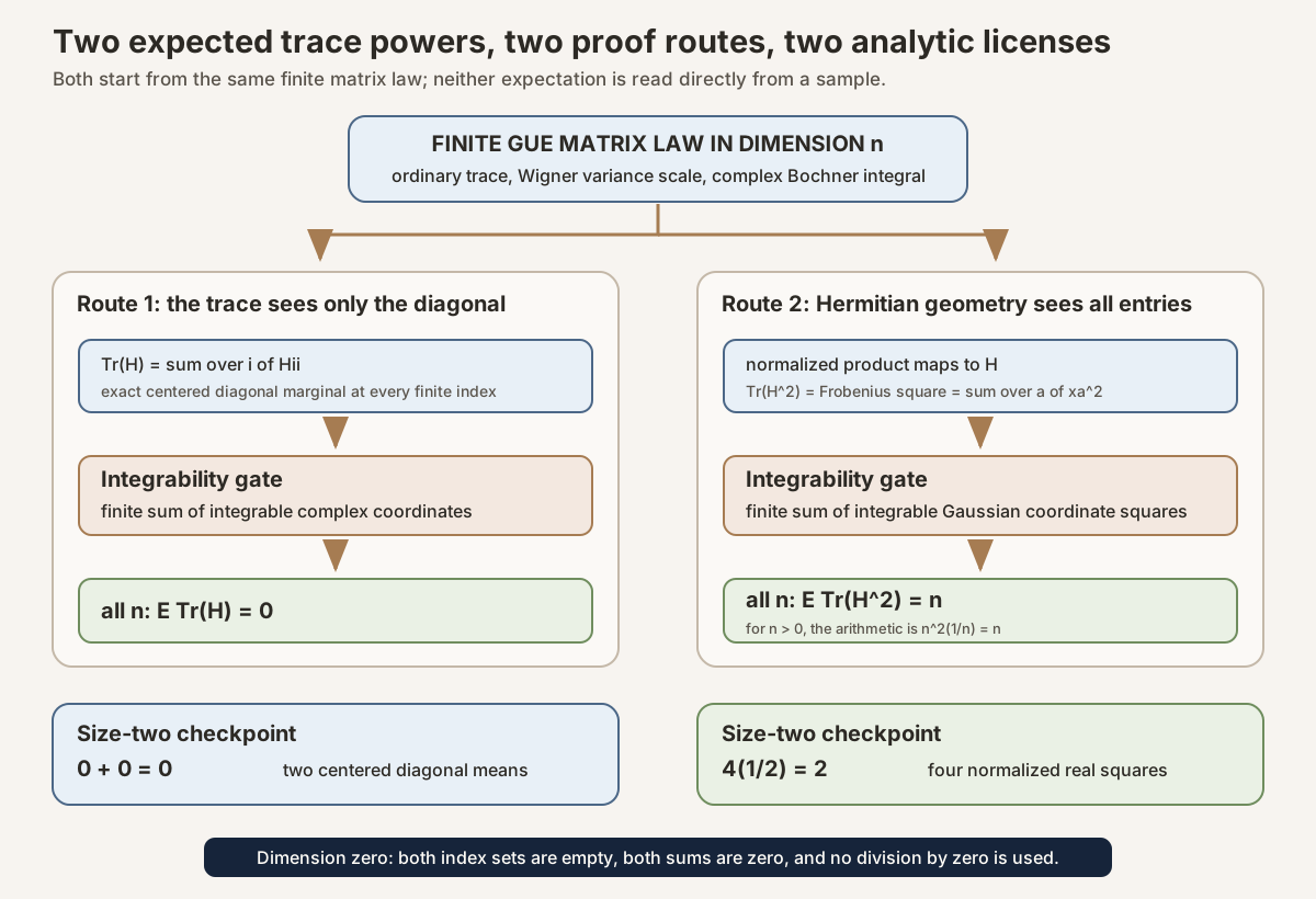
The left route exploits how little the first power contains. Trace is already a finite diagonal sum, so exact centered marginal laws solve the probability problem.
The right route exploits how much the second power contains. Direct entrywise expansion would produce diagonal squares and paired off-diagonal terms. The Hermitian and Frobenius geometry developed in RMT-07 and the normalized coordinate isometry from RMT-08 compress that expansion into a sum of ordinary real squares.
Both routes end in a complex Bochner integral. The codomain does not change merely because the values happen to be real on Hermitian matrices.
Base camp zero: fix every object and convention
For \(n\in\mathbb N\), let
\[ \mu_n=\operatorname{GUE.matrixLaw}(n) \]be the repository’s probability measure on \(\operatorname{Matrix}(\operatorname{Fin}(n),\operatorname{Fin}(n),\mathbb C)\). The phrase ambient matrix law means that the measure lives on all complex matrices of that size, even though RMT-07 proved that it gives full mass to the Hermitian subset.
For a nonnegative integer \(k\), define the pointwise observable
\[ T_k(H)=\operatorname{Tr}(H^k). \]RMT-01 already proved that \(T_k\) is measurable. RMT-09 specializes to \(k=1\) and \(k=2\), proves each \(T_k\) integrable under \(\mu_n\), then evaluates
\[ \int T_k(H)\,\mathrm d\mu_n(H). \]Three conventions are fixed:
- the trace is ordinary, not divided by dimension;
- the GUE law is Wigner scaled, with positive-dimensional variance scale \(s_n=1/n\); and
- the zero-dimensional variance scale is explicitly \(s_0=0\).
The project’s normalization ledger is therefore part of the theorem, not background typography.
Base camp one: why integrability is not bookkeeping
The complex Bochner integral
The Bochner integral extends integration from real-valued functions to functions with values in a Banach space, a complete normed vector space. The complex numbers form such a space. For a function \(f:X\to\mathbb C\) on a measure space \((X,\mu)\), integrability combines two conditions (Mathlib contributors):
- \(f\) is strongly measurable after changing it on a null set if necessary;
- its norm has finite integral,
For finite-dimensional complex targets, familiar measurable functions satisfy the strong-measurability side under the standard Borel structures. The norm bound remains a genuine analytic obligation.
Mathlib represents the property as
MeasureTheory.Integrable f μ
and the Bochner integral as
∫ x, f x ∂μ
The integral is totalized: if the function is not integrable, its definition returns zero (Mathlib contributors). This design makes the operation available without partial terms, but it sharpens our proof discipline. The equation
\[ \int f\,\mathrm d\mu=0 \]does not alone tell a reader whether \(f\) has mean zero or whether the totalized nonintegrable branch was reached. RMT-09 publishes the integrability theorem first in each pair.
Lean bridge: license the first expected trace
MeasureTheory.Integrable (RandomMatrix.tracePower (id : Matrix (Fin n) (Fin n) ℂ → Matrix (Fin n) (Fin n) ℂ) 1) (GUE.matrixLaw n)MeasureTheory.Integrableis the analytic license, not the value of the integral.tracePower … 1is the complex-valued function \(H\mapsto\operatorname{Tr}(H^1)\).- The long
idannotation tells Lean that the sample itself is the matrix-valued random variable. GUE.matrixLaw nsupplies the measure under which norm integrability is proved.- The exact theorem is
GUE.integrable_tracePower_one.
Run boundary. This proposition imports Mathlib’s Bochner integral and the project GUE law. Check it through the full project module probe below, not with the standalone integer worksheet.
Measurability is necessary but weaker
Measurability lets us form a pushforward distribution and discuss the
integral. It does not control tail size. A real function can be measurable and
have infinite first absolute moment. Therefore RMT-01’s measurable
tracePower API could not accurately be described as a moment API.
The boundary is now explicit:
| Layer | Question | RMT status |
|---|---|---|
| Pointwise algebra | What is \(\operatorname{Tr}(H^k)\)? | Defined for every finite matrix |
| Measurability | Is the observable measurable? | Checked for every finite power |
| Integrability | Is its norm integrable under this law? | Now checked for powers one and two of finite GUE |
| Expectation | What is its complex integral under the probability law? | Now evaluated exactly for powers one and two |
| Spectral limit | What happens as dimension grows? | Not formalized |
Pushforward transport has two gates
Let \(F:X\to Y\) be measurable, let \(\nu\) be a source measure on \(X\), and let \(\mu\) be its pushforward \(F_*\nu\). For a suitable \(g:Y\to\mathbb C\), the change-of-variables identity reads
\[ \int_Y g(y)\,\mathrm d(F_*\nu)(y) =\int_X g(F(x))\,\mathrm d\nu(x). \]Mathlib’s integral_map supplies this identity under the relevant
almost-everywhere measurability hypotheses. Separately,
integrable_map_measure relates integrability of \(g\) under the
pushforward to integrability of \(g\circ F\) under the source measure.
(Mathlib contributors)
RMT-09 uses both layers for the second power. Proving only the integral rewrite would not publish the required analytic license. Proving only source integrability would not calculate the target expectation.
Camp one: the first trace reads the diagonal
For every \(n\)-by-\(n\) matrix \(H\),
\[ \operatorname{Tr}(H)=\sum_{i\in\operatorname{Fin}(n)}H_{ii}. \]No Hermitian assumption is needed for this algebraic identity. Under finite
GUE, however, every diagonal entry is real almost surely and has the exact
centered Cartesian complex Gaussian law whose real variance is \(s_n\) and
imaginary variance is zero. The earlier theorem
matrixLaw_diagonal_hasLaw packages this statement for each index
\(i\) (Mathlib contributors).
That marginal law supplies two facts needed here:
- \(H\mapsto H_{ii}\) is integrable under \(\mu_n\);
- its complex mean is zero.
Because the diagonal index is finite, integrability is closed under the sum:
\[ \operatorname{Integrable} \left(H\mapsto\sum_iH_{ii}\right). \]Then finite linearity of the Bochner integral gives
\[ \begin{aligned} \int\operatorname{Tr}(H)\,\mathrm d\mu_n(H) &=\sum_i\int H_{ii}\,\mathrm d\mu_n(H)\\ &=\sum_i0\\ &=0. \end{aligned} \]This proof is deliberately local. It does not use the full normalized real product representation, the unitary-invariance theorem, or independence among entries. Exact centered diagonal marginals are sufficient.
Lean bridge: evaluate the first expected trace
∫ H, RandomMatrix.tracePower (id : Matrix (Fin n) (Fin n) ℂ → Matrix (Fin n) (Fin n) ℂ) 1 H ∂GUE.matrixLaw n = 0∫ H, … ∂GUE.matrixLaw nis Lean’s binder syntax for the Bochner integral over matrices.- The final
Hevaluates the trace-power function at the bound matrix. = 0is a complex equality; the preceding integrability theorem prevents the totalized nonintegrable zero from being misread as a mean.- The source expands trace into a finite diagonal sum and uses
(matrixLaw_diagonal_hasLaw n i).mean_eqat each index. - The exact theorem is
GUE.integral_tracePower_one.
Run boundary. The standalone worksheet checks \(2+(-1)=1\) for one sample and a zero centered-mean ledger. The law-level integral is a full project check.
The empty first sum
When \(n=0\), Fin 0 has no elements. Matrix trace is the sum over
the empty diagonal, so it is zero pointwise. The same generic finite-sum proof
therefore gives integrability and zero integral. No special public theorem or
division argument is needed.
Camp two: Hermitian trace square is Frobenius energy
The second power sees off-diagonal entries, but Hermiticity organizes them. Write \(H^*\) for conjugate transpose. If \(H\) is Hermitian, then \(H^*=H\), equivalently \(H_{ji}=\overline{H_{ij}}\). Expand trace and matrix multiplication:
\[ \begin{aligned} \operatorname{Tr}(H^2) &=\sum_i(H^2)_{ii}\\ &=\sum_{i,j}H_{ij}H_{ji}\\ &=\sum_{i,j}H_{ij}\overline{H_{ij}}\\ &=\sum_{i,j}|H_{ij}|^2\\ &=\lVert H\rVert_F^2. \end{aligned} \]The last expression is the squared Frobenius norm . It is real and nonnegative, then included into ℂ in the theorem statement (Mathlib contributors).
The private Lean helper trace_sq_hermitianToMatrix proves this
pointwise identity on the intrinsic Hermitian Euclidean carrier. Rather than
expanding two finite sums again, it consumes RMT-07’s checked identity between
the Frobenius inner product and
\(\operatorname{Tr}(X^*Y)\), specializes to \(X=Y=H\), and rewrites \(H^*=H\).
This is an important reuse boundary. The moment module does not re-prove the geometry from raw entries, and the geometry module makes no probability claim.
Lean bridge: turn Hermitian trace-square into energy
Matrix.trace ((RandomMatrix.hermitianToMatrix H) ^ 2) = (‖H‖ ^ 2 : ℂ)Hhas typeRandomMatrix.HermitianEuclidean n, so Hermiticity is carried by the value itself.hermitianToMatrixforgets the subtype proof and exposes the ambient entries.^ 2on the left is matrix multiplication;‖H‖ ^ 2on the right is a real norm square.(… : ℂ)coerces that real energy into the complex trace codomain.- This is the private checked helper
trace_sq_hermitianToMatrix, derived from RMT-07’s publicRandomMatrix.inner_frobenius_eq_trace.
Run boundary. Because the helper is private, it is audited by checking the whole RMT-09 source leaf. The standalone worksheet checks its displayed \(n=2\) instance, \(15=15\).
Camp three: move the law to normalized real coordinates
RMT-08 introduced the finite real index
\[ \mathcal I_n =\operatorname{Fin}(n) \sqcup I_n^{\lt} \sqcup I_n^{\lt}, \]where \(I_n^{\lt}\) is the set of strict-upper positions. Its three regions hold the diagonal, normalized upper-real, and normalized upper-imaginary coordinates. The normalized assembly map decodes a real function \(x:\mathcal I_n\to\mathbb R\) into a Hermitian matrix by keeping the diagonal and dividing both upper components by \(\sqrt2\).
The factor \(\sqrt2\) is forced by reflection. Every strict-upper entry appears again as its conjugate below the diagonal. Raw upper real and imaginary parts therefore carry twice the Frobenius weight of a diagonal coordinate. The normalization makes assembly a real linear isometry:
\[ \lVert H(x)\rVert_F^2 =\sum_{a\in\mathcal I_n}x_a^2. \]RMT-08 also proved equality of the complete normalized product law with the
earlier coordinate-built GUE law. RMT-09 exposes the direct composite
normalizedRealMatrixSample n privately and proves
This is an equality of whole measures, not a statement that the coordinates merely have matching variances. It licenses the pushforward integration step.
Lean bridge: transport the complete normalized product
(gaussianProductMeasure (fun _ : HermitianRealIndex n ↦ 0) (fun _ ↦ GUE.varianceScale n)).map RandomMatrix.realToHermitianCoordinates = GUE.coordinateMeasure ngaussianProductMeasurebuilds the finite joint law; the two functions provide mean zero and common variance at every index.HermitianRealIndex nhas diagonal, normalized upper-real, and normalized upper-imaginary sectors..mapis pushforward of the entire measure, not a list of marginal variance statements.realToHermitianCoordinatesdivides both upper sectors by \(\sqrt2\) and pairs them into complex entries.- The exact predecessor theorem is
GUE.map_realToHermitianCoordinates_gaussianProduct.
Run boundary. This predecessor theorem and RMT-09’s private composite to
matrixLaw n both require the pinned Mathlib project.
Combining the measure equality with the pointwise norm identity gives
\[ T_2(H(x)) =\operatorname{Tr}(H(x)^2) =\left(\sum_{a\in\mathcal I_n}x_a^2:\mathbb R\right) \]viewed in ℂ. In Lean, the private theorem
tracePower_two_normalizedRealMatrixSample is exactly this
deterministic bridge.
Camp four: prove the sum of squares integrable
Fix one coordinate \(a\in\mathcal I_n\). Under the finite product measure, evaluation at \(a\) has the centered real Gaussian law \(N(0,s_n)\). The project’s exact real Gaussian API supplies finite second-power membership and hence integrability of \(x_a^2\):
\[ \int |x_a^2|\,\mathrm d\rho_n(x)\lt\infty, \]where \(\rho_n\) denotes the normalized real product measure.
Because \(\mathcal I_n\) is finite, the whole sum of squares is integrable:
\[ x\longmapsto\sum_{a\in\mathcal I_n}x_a^2. \]The Lean proof packages the scalar fact in the private helper
centeredGaussian_integrable_sq, applies it to each evaluation
marginal, and uses integrable_finsetSum. It then converts the real
integrable function to its complex inclusion and transfers integrability
through the measurable normalized assembly map.
The target statement is not about the coordinate source measure. The theorem
integrable_tracePower_two explicitly concludes integrability of
tracePower id 2 under matrixLaw n. The proof passes
through integrable_map_measure and the pointwise bridge, so the
analytic result lands on the public ambient law.
Lean bridge: license the second expected trace
MeasureTheory.Integrable (RandomMatrix.tracePower (id : Matrix (Fin n) (Fin n) ℂ → Matrix (Fin n) (Fin n) ℂ) 2) (GUE.matrixLaw n)- The only visible change from the first integrability proposition is the
power
2; the proof route is completely different. integrable_map_measuremoves the target question to normalized coordinate space.integrable_finsetSumassembles the finite family of integrable coordinate squares..ofRealincludes the real square sum into the complex codomain.- The exact theorem is
GUE.integrable_tracePower_two.
Run boundary. The worksheet checks finite identities only. The norm-tail control and pushforward transfer are checked by the primary full project module.
Why no independence calculation appears
The source law is a product, so its coordinates are indeed jointly independent. But after the Frobenius identity, the observable is a finite sum of one-coordinate squares. Linearity of integration gives
\[ \int\sum_a x_a^2\,\mathrm d\rho_n =\sum_a\int x_a^2\,\mathrm d\rho_n \]without any independence hypothesis. Independence becomes essential when an observable contains products of distinct coordinates and one wants to factor their expectations. No such cross terms survive here.
The exact product-law theorem still matters. It establishes the source measure and the evaluation marginals used in the calculation. The narrow claim is that the final integration step does not invoke an independence factorization.
Camp five: count the coordinates and close the normalization
For a centered real Gaussian \(Z\sim N(0,s_n)\),
\[ \mathbb E[Z^2]=s_n. \]RMT-09 derives this from the earlier exact mean and variance theorems. Its
private helper centeredGaussian_integral_sq does not integrate a
density by hand.
Therefore
\[ \begin{aligned} \int\sum_{a\in\mathcal I_n}x_a^2\,\mathrm d\rho_n(x) &=\sum_{a\in\mathcal I_n}s_n\\ &=|\mathcal I_n|s_n. \end{aligned} \]RMT-08 built a finite equivalence
\[ \mathcal I_n\simeq\operatorname{Fin}(n)\times\operatorname{Fin}(n). \]The moment module uses that equivalence to prove
\[ |\mathcal I_n|=n^2. \]Now the normalization arithmetic separates cleanly into two branches.
For \(n=0\), the coordinate index is empty and \(s_0=0\), so
\[ |\mathcal I_0|s_0=0. \]For a successor dimension, hence positive \(n\), the variance scale is \(s_n=1/n\), so
\[ |\mathcal I_n|s_n =n^2\frac1n =n. \]The private theorem card_mul_varianceScale implements exactly this
zero/successor split. The public theorem needs no assumption \(0\lt n\).
Lean bridge: close the exact second expectation
∫ H, RandomMatrix.tracePower (id : Matrix (Fin n) (Fin n) ℂ → Matrix (Fin n) (Fin n) ℂ) 2 H ∂GUE.matrixLaw n = (n : ℂ)integral_mapmoves the target integral through the normalized real matrix sample map.integral_congr_aereplaces the composed trace-square by the pointwise coordinate square sum.integral_finsetSumuses scalar Gaussian second moments; it does not factor a product of distinct coordinates.Fintype.card (HermitianRealIndex n)becomes \(n^2\), andvarianceScale ncontributes \(1/n\) in positive dimension.(n : ℂ)makes the complex codomain explicit.- The exact theorem is
GUE.integral_tracePower_two.
Run boundary. This is the full project RMT-09 endpoint. The standalone worksheet checks the \(n=2\) arithmetic \(4(1/2)=2\), not the measure integral.
A two-by-two audit
For \(n=2\), a Hermitian matrix has two real diagonal entries and one complex strict-upper entry. The normalized real ledger therefore has four directions:
\[ d_1,\quad d_2,\quad \sqrt2\operatorname{Re}(u),\quad \sqrt2\operatorname{Im}(u). \]Each normalized coordinate has variance \(1/2\). Their squared sum has expected value
\[ 4\cdot\frac12=2, \]which matches the theorem’s right side. In displayed matrix entries, \(\operatorname{Re}(u)\) and \(\operatorname{Im}(u)\) each have variance \(1/4\), and the conjugate lower entry supplies the second Frobenius copy. This check is small enough to do by hand and catches the most common factor-of-two error.
The complete normalization ledger
| Convention | Dimension zero | Positive dimension | Role in RMT-09 |
|---|---|---|---|
| Matrix index | Fin 0 is empty | Fin n has \(n\) indices | Controls trace sums |
| Variance scale \(s_n\) | \(0\) | \(1/n\) | Common variance of normalized real coordinates |
| Diagonal entry | Unique empty family | Real centered Gaussian with variance \(1/n\) | First moment and part of second |
| Strict-upper real part | Unique empty family | Centered Gaussian with variance \(1/(2n)\) | Displayed entry convention |
| Strict-upper imaginary part | Unique empty family | Centered Gaussian with variance \(1/(2n)\) | Displayed entry convention |
| Normalized upper coordinates | Unique empty family | Multiply displayed components by \(\sqrt2\) | Restores common variance \(1/n\) |
| Number of normalized real coordinates | \(0\) | \(n^2\) | One per ambient matrix position via a finite equivalence |
| Trace convention | Ordinary trace | Ordinary trace | Produces second moment \(n\), not \(1\) |
| Density exponent | Not defined or used | Classical context would use \(-n\operatorname{Tr}(H^2)/2\) | Explicit nonclaim |
| Spectral scale | Empty spectrum | Order-one interpretation is classical context | No finite or asymptotic spectral theorem follows |
The ledger explains three formulas that can otherwise look contradictory. Diagonal entries have variance \(1/n\), displayed upper real and imaginary parts each have variance \(1/(2n)\), and every normalized real coordinate has variance \(1/n\). They describe the same law in different coordinate systems.
The four checked declarations
The public module has no new definition or instance. Its complete API is:
theorem GUE.integrable_tracePower_one (n : ℕ) :
    MeasureTheory.Integrable
      (RandomMatrix.tracePower
        (id : Matrix (Fin n) (Fin n) ℂ → Matrix (Fin n) (Fin n) ℂ) 1)
      (GUE.matrixLaw n)

theorem GUE.integral_tracePower_one (n : ℕ) :
    ∫ H : Matrix (Fin n) (Fin n) ℂ,
        RandomMatrix.tracePower id 1 H ∂GUE.matrixLaw n = 0

theorem GUE.integrable_tracePower_two (n : ℕ) :
    MeasureTheory.Integrable
      (RandomMatrix.tracePower
        (id : Matrix (Fin n) (Fin n) ℂ → Matrix (Fin n) (Fin n) ℂ) 2)
      (GUE.matrixLaw n)

theorem GUE.integral_tracePower_two (n : ℕ) :
    ∫ H : Matrix (Fin n) (Fin n) ℂ,
        RandomMatrix.tracePower id 2 H ∂GUE.matrixLaw n = (n : ℂ)
All four compile under Lean 4.32.0 with the repository’s pinned Mathlib 4.32.0
revision. The theorem axiom audit reports only propext,
Classical.choice, and Quot.sound, the standard logical
and quotient principles inherited from Lean and Mathlib. There are no project
axioms or proof holes.
Declaration map
| Declaration | Checked result | Main proof route | Deliberate boundary |
|---|---|---|---|
GUE.integrable_tracePower_one | The first trace-power observable is complex Bochner integrable under matrixLaw n | Expand trace as a finite diagonal sum; use integrability from each exact diagonal marginal law | No value of the integral yet |
GUE.integral_tracePower_one | The first complex integral is zero | Move integral through the finite sum; replace every diagonal mean by zero | No independence or symmetry argument |
GUE.integrable_tracePower_two | The second trace-power observable is complex Bochner integrable under matrixLaw n | Rewrite the matrix law as a normalized real product pushforward; prove a finite sum of Gaussian squares integrable; transfer through the map | No density or eigenvalue route |
GUE.integral_tracePower_two | The second complex integral is the dimension | Apply integral_map, rewrite pointwise to the coordinate square sum, integrate scalar second moments, count coordinates, split zero from successor dimension | No higher moment, concentration, or limit |
Private scaffolding and why it remains private
The module contains private helpers for the deterministic trace-square identity, scalar centered-Gaussian square integrability and expectation, the normalized real sample map, the exact pushforward comparison, the coordinate square-sum identity, finite-sum integration, coordinate cardinality, and normalization arithmetic.
These are proof architecture, not a competing public theory. The reusable geometric maps and Gaussian law interfaces already live in earlier modules. Keeping the local compositions private leaves the public API focused on the four analytic facts downstream code needs.
The second integrability proof in Lean-shaped steps
The proof of integrable_tracePower_two follows this chain:
- rewrite
matrixLaw nas the map of the normalized real Gaussian product bynormalizedRealMatrixSample n; - invoke
integrable_map_measurewith measurability of the sample map and strong measurability oftracePower id 2; - use the pointwise equality between the composed trace power and the complex inclusion of the real coordinate square sum;
- prove the real finite sum integrable coordinate by coordinate; and
- transfer integrability through the real-to-complex inclusion.
The integral theorem repeats the law rewrite, uses integral_map,
uses integral_congr_ae for the pointwise square-sum identity,
commutes real inclusion with integration, and applies the exact finite sum and
cardinality calculation.
Why eigenvalues are unnecessary here
For a Hermitian matrix with real eigenvalues \(\lambda_1,\ldots,\lambda_n\), the spectral theorem classically gives
\[ \operatorname{Tr}(H^k)=\sum_{r=1}^n\lambda_r^k. \]This is the finite algebraic doorway into the classical trace-moment method (Anderson, Guionnet, and Zeitouni; Tao; Wigner).
That formula motivates the name spectral moment, but formalizing it at the law level would require more infrastructure: a measurable eigenvalue enumeration or multiset, multiplicity bookkeeping, and a measurable empirical spectral measure. None is needed for \(k=1\) or \(k=2\).
The first identity is visible from diagonal entries. The second is visible from Hermitian Frobenius geometry. Entry coordinates already carry exact measurable laws, so routing through eigenvalues would lengthen the proof and introduce choices irrelevant to these two finite results.
This is not an argument against eigenvalues. They are the natural next layer for empirical spectral measures and spectral statistics. It is an argument for proving each theorem at the weakest sufficient interface.
Why a density is unnecessary here
For positive \(n\), the classical Wigner-scaled GUE density is proportional to
\[ \exp\!\left(-\frac n2\operatorname{Tr}(H^2)\right) \]relative to a chosen Lebesgue measure on the real vector space of Hermitian matrices (Guionnet). One could in principle integrate the first two trace powers against that density.
The repository has not formalized that density, its normalizing constant, or the reference volume. RMT-09 does not need them. The coordinate construction already provides a probability measure, RMT-08 identifies it with a scaled intrinsic Gaussian, and scalar Gaussian moment theorems evaluate the required finite sums.
Avoiding a density also keeps the dimension-zero case well-defined. An empty finite product and a Dirac law are already meaningful there, while formulas involving positive-dimensional Lebesgue density require a separate convention.
Physics window: what the second identity suggests
For a Hermitian Hamiltonian, \(\operatorname{Tr}(H^2)\) is the sum of squared energy eigenvalues. The checked expectation \(n\) means that the expected ordinary average per eigenvalue is one for positive dimension:
\[ \mathbb E\!\left[\frac1n\operatorname{Tr}(H^2)\right]=1. \]This is consistent with the order-one spectral scale intended by Wigner normalization. It is one calibration check behind the semicircle regime.
The Lean theorem is narrower. It states the ordinary-trace identity for each finite \(n\), including zero. It does not define random energy eigenvalues, prove that an empirical measure exists measurably, or show convergence to the semicircle distribution. The normalized positive-dimensional corollary above is explanatory mathematics and requires \(0\lt n\); it is not one of the four public declarations.
Common wrong turns
Calling measurability a moment theorem
A measurable trace power may have an infinite norm integral. Publish an
Integrable theorem before interpreting the Bochner integral as a
finite expectation.
Forgetting that the Bochner integral is totalized
An integral equation with value zero is not by itself evidence of mean zero in Mathlib. The nonintegrable branch also evaluates to zero by definition.
Using raw upper-entry coordinates in the norm square
Every strict-upper entry is reflected below the diagonal. Raw upper real and imaginary parts have Frobenius weight two. The normalized real coordinates absorb that weight through the square-root-of-two correction.
Assigning normalized-coordinate variance to displayed upper components
The normalized upper coordinates have variance \(1/n\). The displayed real and imaginary parts after decoding each have variance \(1/(2n)\). Confusing the two descriptions doubles the second moment.
Expanding cross terms and demanding independence
The Hermitian trace-square identity becomes a sum of coordinate squares, not the square of a coordinate sum. Linearity of expectation is sufficient. There are no distinct-coordinate products to factor.
Dividing by dimension before handling zero
The public result uses ordinary trace and includes \(n=0\). Only a later positive-dimensional corollary may divide by \(n\).
Inferring a semicircle law from two moments
Two exact finite moments do not determine an arbitrary probability law and do not establish convergence of empirical spectral measures. Higher moments, tightness or another convergence framework, and measurable spectral data are separate prerequisites.
Worked audit checklist
Before accepting a finite random-matrix moment formula, ask:
- What is the exact matrix law and on which measurable space does it live?
- Is the trace ordinary or normalized?
- Is the matrix itself scaled, and where does the dimension enter?
- Is the trace-power observable measurable?
- Has its norm integrability been proved under this law?
- Is the displayed integral real-valued or complex-valued?
- If a pushforward is used, were both measurability and integrability moved through it?
- Are entry variances stated for displayed entries or orthonormal coordinates?
- Does a coordinate count include the diagonal and both upper real directions?
- Is dimension zero included, excluded, or assigned a separate convention?
- Did the proof actually use independence, or only scalar marginals and linearity?
- Does the conclusion concern one finite dimension or a limit?
RMT-09 answers each question explicitly.
Exercises from trailhead to summit
Trailhead
- Let \[ H=\begin{bmatrix}a&u\\\overline u&b\end{bmatrix} \] with \(a,b\in\mathbb R\) and \(u\in\mathbb C\). Expand \(\operatorname{Tr}(H^2)\) and verify \(a^2+b^2+2|u|^2\).
- Substitute \(u=(x+iy)/\sqrt2\). Show that the same expression becomes \(a^2+b^2+x^2+y^2\).
- If all four normalized coordinates are centered with variance \(1/2\), evaluate the expected sum without using independence.
Mid-mountain
- Prove on paper that a finite sum of integrable complex-valued functions is integrable and that its Bochner integral is the sum of their integrals.
- Give an example of a measurable real random variable that is not integrable. Explain what Mathlib’s totalized integral returns and why the corresponding equation should not be advertised as an expectation theorem.
- Write the change-of-variables identity for a pushforward measure and list the measurability hypotheses on the map and the integrand. Then state the separate integrability equivalence needed in the RMT-09 proof.
- Count the diagonal, strict-upper real, and strict-upper imaginary regions directly and verify \(n+2\binom n2=n^2\). Compare this arithmetic proof with using a finite equivalence to all ordered matrix positions.
Summit
- For positive \(n\), derive the expected normalized second trace moment from the checked ordinary-trace theorem. Explain why the proof cannot be specialized to \(n=0\).
- Expand \(\operatorname{Tr}(H^3)\) in entries. Identify where products of distinct coordinates appear and why centeredness and independence become more consequential than they were for the second power.
- Design the next formal interface for empirical spectral measures. State which parts require measurable eigenvalue data and which finite trace identities could be reused after that bridge is checked.
- Compare a density-based proof of the second moment with the product-law proof used here. List the extra reference-measure, normalization, and change-of-variables obligations introduced by the density route.
Full project checks
Inspect the geometry and normalized-law predecessors
Full project check: predecessor project module plus Mathlib. Place this probe in a temporary project scratch file:
import NonlinearDynamics.Random.RandomMatrices.GaussianUnitaryEnsembleInvariance

open Matrix MeasureTheory ProbabilityTheory
open scoped Matrix NNReal ENNReal RealInnerProductSpace
open NonlinearDynamics.Random

#check HermitianRealIndex
#check GUE.varianceScale
#check RandomMatrix.inner_frobenius_eq_trace
#check RandomMatrix.normalizedHermitianAssembly_inner
#check GUE.map_realToHermitianCoordinates_gaussianProduct
#check GUE.matrixLaw_eq_map_hermitianToMatrix_intrinsicLaw
#check elaborates each exact declaration and displays
its type. It does not sample a matrix or evaluate an expectation. The full
project command rendered below checks the authoritative predecessor source
file.
cd formalization
lake env lean -DwarningAsError=true NonlinearDynamics/Random/RandomMatrices/GaussianUnitaryEnsembleInvariance.lean
Resource note: this exact file uses the repository's
pinned Lean and Mathlib dependencies. Initial project setup can require
substantial disk space and build time. For a lightweight first step on
macOS or Linux, use the page's standalone Lean-core or Std
tutorial.
Inspect all four RMT-09 endpoints
Full project check: primary project module plus Mathlib. Type this exact probe in a temporary project scratch file:
import NonlinearDynamics.Random.RandomMatrices.GaussianUnitaryEnsembleMoments

open Matrix MeasureTheory ProbabilityTheory
open scoped Matrix NNReal ENNReal RealInnerProductSpace
open NonlinearDynamics.Random

#check RandomMatrix.tracePower
#check RandomMatrix.measurable_tracePower
#check GUE.integrable_tracePower_one
#check GUE.integral_tracePower_one
#check GUE.integrable_tracePower_two
#check GUE.integral_tracePower_two
The first two checks expose the observable and its earlier measurability gate. The final four are the complete public API of RMT-09. The full project command below checks the whole leaf with the repository’s pinned toolchain and dependencies.
cd formalization
lake env lean -DwarningAsError=true NonlinearDynamics/Random/RandomMatrices/GaussianUnitaryEnsembleMoments.lean
Resource note: this exact file uses the repository's
pinned Lean and Mathlib dependencies. Initial project setup can require
substantial disk space and build time. For a lightweight first step on
macOS or Linux, use the page's standalone Lean-core or Std
tutorial.
Passing technical checks does not change pro_reviewed: false or
complete the pending human mathematical, editorial, and accessibility review.
What has and has not been proved
| Topic | Checked status after RMT-09 |
|---|---|
| Measurability of every finite trace power | Checked earlier |
| Integrability of the first GUE trace power | Checked for every natural dimension |
| Exact first complex integral | Checked and equal to zero |
| Integrability of the second GUE trace power | Checked for every natural dimension |
| Exact second complex integral | Checked and equal to the matrix dimension |
| Dimension-zero behavior | Included in all four public theorems |
| Equality of Hermitian trace square and Frobenius norm square | Checked privately here from reusable RMT-07 geometry |
| Exact normalized product pushforward | Checked earlier and consumed here |
| Higher expected trace powers | Not checked |
| Variance or concentration of trace powers | Not checked |
| Measurable eigenvalue enumeration | Not checked |
| Empirical spectral measure | Not defined |
| Joint eigenvalue density | Not checked |
| Semicircle law or any large-dimension convergence | Not checked |
| Local spacing statistics or universality | Not checked |
| Quantum dynamics | Not checked |
The finite identities are exact and useful. Their narrowness is a strength: the next spectral layer can consume them without inheriting an unspoken density or positivity convention.
Where to continue
The finite matrix trace moment glossary entry gives a compact operational definition and normalization audit. Read trace-power observable for the earlier measurability boundary and matrix trace for the underlying finite algebra.
From Normalized Hermitian Coordinates to Gaussian Unitary Ensemble Invariance constructs the exact real product pushforward consumed by the second-moment proof. Intrinsic Hermitian Gaussian Symmetry and Matrix-Law Support develops the Frobenius geometry, while Finite GUE from Independent Gaussian Coordinates fixes the entrywise Wigner law.
RMT-10A supplies the algebraic finite-spectrum interface and a zero-aware empirical spectral measure. Read Finite Hermitian Spectra and Empirical Measures for that continuation. RMT-10B discharges its measurability premise, and Finite Gaussian Unitary Ensemble Empirical Spectral Laws and Normalized Moments then constructs the unconditional law and transports the two exact trace expectations into normalized sample moments. No spectral limit is claimed.
References
Mathlib contributors.
Bochner integral,
Mathlib 4 documentation. This official API defines the Banach-valued integral,
its totalized nonintegrable branch, linearity, finite sums, and
integral_map.
Mathlib contributors.
Integrable functions
and
pushforward of a measure,
Mathlib 4 documentation. These official references document the
Integrable interface, integrable_map_measure, and the
measure-map semantics used to transfer the second observable from normalized
coordinates to ambient matrices.
Mathlib contributors. Real Gaussian distributions, multivariate Gaussian distributions, and finite product measures, Mathlib 4 documentation. These official pages provide the exact centered Gaussian mean and variance results, finite moments, and product-coordinate marginals used in the proof.
Mathlib contributors. Matrix trace, Hermitian matrices, and Pi-L2 Euclidean spaces, Mathlib 4 documentation. These official algebraic and geometric APIs underlie the trace expansion, Hermitian conjugate symmetry, and normalized-coordinate norm calculation.
Greg W. Anderson, Alice Guionnet, and Ofer Zeitouni. An Introduction to Random Matrices, Cambridge University Press, 2010. Chapters 2 and 3 give standard treatments of Wigner matrices, trace moments, Gaussian ensembles, and their spectral interpretation. The project’s exact entry variances and ordinary-trace convention are stated independently because literature normalizations differ.
Terence Tao. Topics in Random Matrix Theory, American Mathematical Society, 2012. This standard monograph develops the moment method and Wigner normalization toward the semicircle law. RMT-09 stops at the first two exact finite identities and does not import its asymptotic conclusions.
Alice Guionnet. Rare Events in Random Matrix Theory, in Proceedings of the International Congress of Mathematicians 2022, volume 2, European Mathematical Society Press, 2022, pp. 1008-1052. Section 1.1.1 records the diagonal variance \(1/n\), upper real and imaginary variances \(1/(2n)\), and invariant density convention for Wigner-scaled GUE. The checked proof here uses the product law, not the density.
Eugene P. Wigner. Characteristic Vectors of Bordered Matrices With Infinite Dimensions, Annals of Mathematics 62 (1955), 548-564. This primary source supplies historical context for the trace-moment route to large random-matrix spectra. Its limiting theorem is not a premise or conclusion of RMT-09.
The exact upstream Lean source audited for this chapter is Mathlib commit
81a5d257,
the revision pinned by formalization/lake-manifest.json.