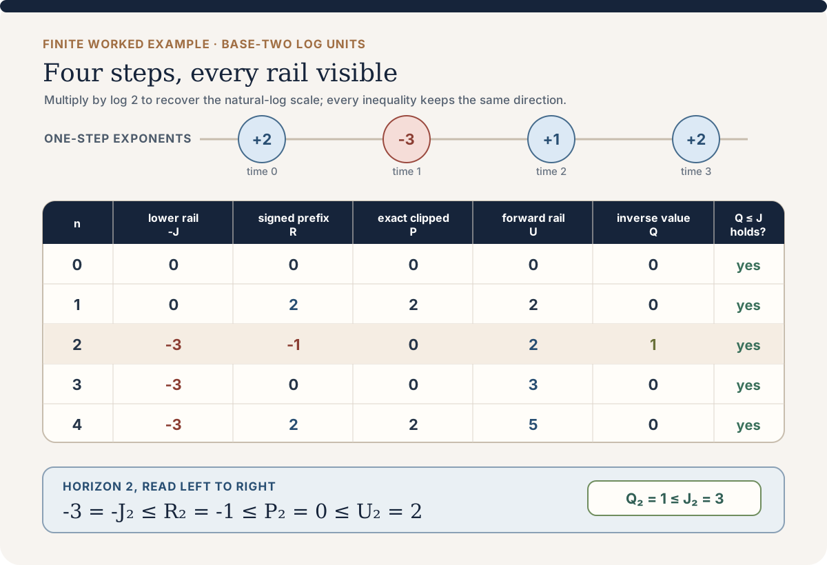
Start with four scalar steps you can audit
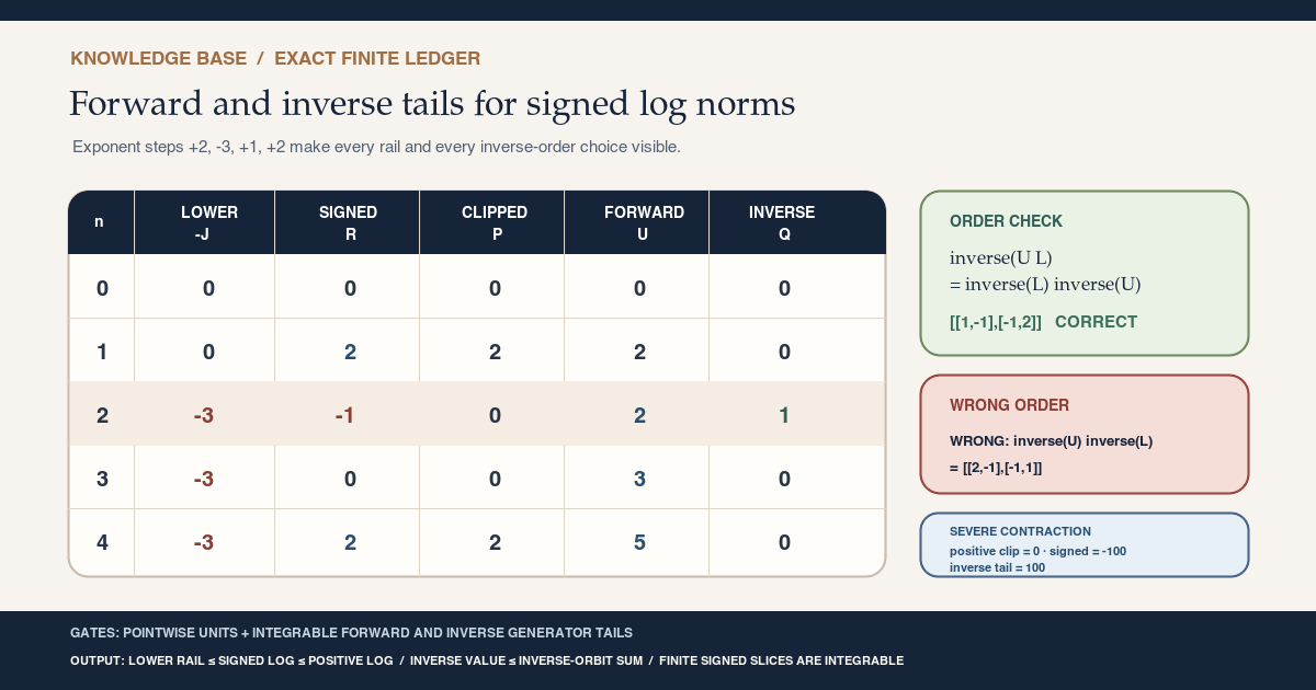
Begin in one dimension, where every matrix is a nonzero scalar and products commute. Use powers of two so every logarithm becomes integer arithmetic. Choose the four generator multipliers
\[ a_0=2^2=4,\qquad a_1=2^{-3}=\frac18,\qquad a_2=2^1=2,\qquad a_3=2^2=4. \]Their base-two log exponents are
\[ (e_0,e_1,e_2,e_3)=(2,-3,1,2). \]For horizon \(n\), multiply the first \(n\) generators and define five quantities:
\[ \begin{aligned} R_n^{(2)} &:=\log_2\left|\prod_{j=0}^{n-1}a_j\right| =\sum_{j=0}^{n-1}e_j,\\ P_n^{(2)} &:=\max(R_n^{(2)},0),\\ U_n^{(2)} &:=\sum_{j=0}^{n-1}\max(e_j,0),\\ Q_n^{(2)} &:=\max(-R_n^{(2)},0),\\ J_n^{(2)} &:=\sum_{j=0}^{n-1}\max(-e_j,0). \end{aligned} \]Here \(R_n^{(2)}\) is the signed log of the whole product, \(P_n^{(2)}\) is the positive log of that product, \(U_n^{(2)}\) is the looser sum of one-step forward positive logs, \(Q_n^{(2)}\) is the positive log of the inverse product, and \(J_n^{(2)}\) is the sum of one-step inverse positive logs. The superscript \((2)\) records the temporary base-two scale. Multiplying every entry by the positive constant \(\log 2\) converts the ledger to the natural logarithms used by Lean without changing any inequality.
| \(n\) | Prefix product | \(R_n^{(2)}\) | \(-J_n^{(2)}\) | \(P_n^{(2)}\) | \(U_n^{(2)}\) | \(Q_n^{(2)}\) |
|---|---|---|---|---|---|---|
| 0 | \(1\) | \(0\) | \(0\) | \(0\) | \(0\) | \(0\) |
| 1 | \(4\) | \(2\) | \(0\) | \(2\) | \(2\) | \(0\) |
| 2 | \(1/2\) | \(-1\) | \(-3\) | \(0\) | \(2\) | \(1\) |
| 3 | \(1\) | \(0\) | \(-3\) | \(0\) | \(3\) | \(0\) |
| 4 | \(4\) | \(2\) | \(-3\) | \(2\) | \(5\) | \(0\) |
Every row verifies the complete chain
\[ -J_n^{(2)} \le -Q_n^{(2)} \le R_n^{(2)} \le P_n^{(2)} \le U_n^{(2)}. \]The checked module uses the sharper middle upper rail \(R_n\le P_n\). Earlier forward-tail integrability results make \(P_n\) integrable by controlling it with the one-step sum represented here by \(U_n^{(2)}\). Keeping both columns prevents two different positive-log objects from being silently identified.
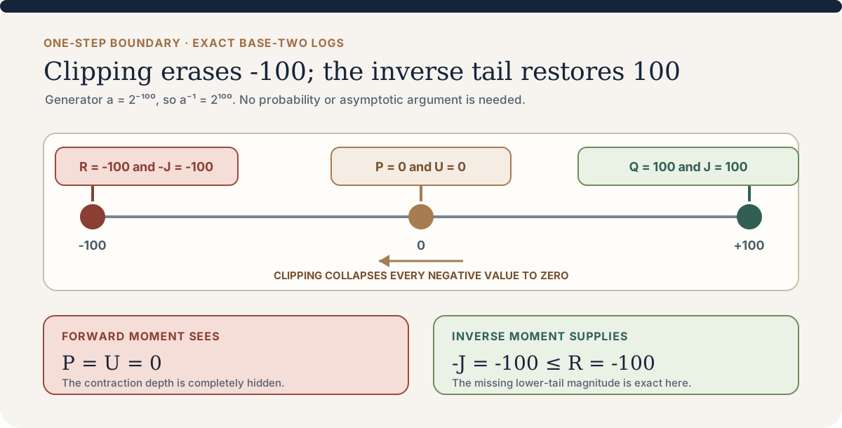
One severe contraction exposes the missing tail
Now take a single generator \(a=2^{-100}\). Its signed log exponent is \(-100\), but its forward positive log is zero:
\[ R_1^{(2)}=-100, \qquad P_1^{(2)}=U_1^{(2)}=0. \]An expansion-only moment sees nothing. The inverse multiplier is \(2^{100}\), so both inverse quantities record the missing magnitude:
\[ Q_1^{(2)}=J_1^{(2)}=100, \qquad -J_1^{(2)}=-100=R_1^{(2)}. \]This is the smallest possible reason that a forward positive-log moment cannot control signed integrability by itself.
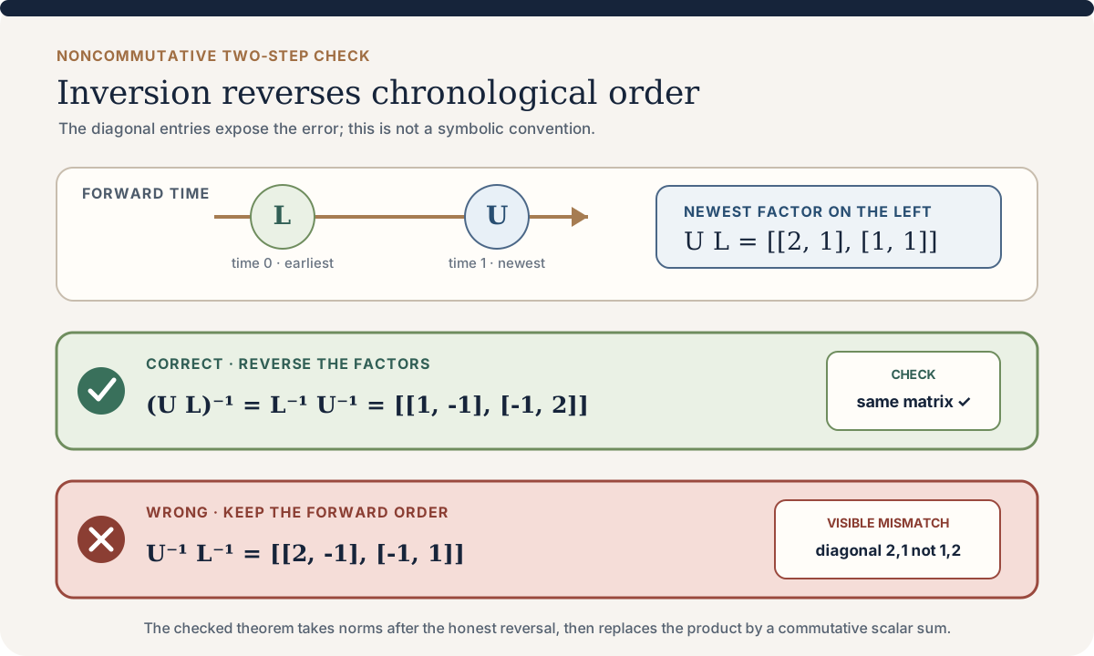
Noncommuting shears determine chronological order
Scalar products hide one matrix issue because scalars commute. Let
\[ U= \begin{bmatrix} 1&1\\ 0&1 \end{bmatrix}, \qquad L= \begin{bmatrix} 1&0\\ 1&1 \end{bmatrix}. \]If the time-zero generator is \(L\) and the time-one generator is \(U\), the newest-factor-left cocycle value is
\[ UL= \begin{bmatrix} 2&1\\ 1&1 \end{bmatrix}. \]Inversion reverses the product:
\[ \begin{aligned} (UL)^{-1} &=L^{-1}U^{-1}\\ &= \begin{bmatrix} 1&-1\\ -1&2 \end{bmatrix}. \end{aligned} \]A direct multiplication checks that this displayed matrix is a two-sided inverse:
\[ \begin{aligned} \begin{bmatrix}1&-1\\-1&2\end{bmatrix} \begin{bmatrix}2&1\\1&1\end{bmatrix} &= \begin{bmatrix}1&0\\0&1\end{bmatrix},\\ \begin{bmatrix}2&1\\1&1\end{bmatrix} \begin{bmatrix}1&-1\\-1&2\end{bmatrix} &= \begin{bmatrix}1&0\\0&1\end{bmatrix}. \end{aligned} \]Keeping the forward order after inversion gives a different matrix:
\[ U^{-1}L^{-1}= \begin{bmatrix} 2&-1\\ -1&1 \end{bmatrix} \ne (UL)^{-1}. \]The inverse factors therefore cannot be advertised as another newest-factor-left cocycle over the same one-sided base.
From the finite ledger to RMT-34
Imagine climbing from a valley where every contraction has been hidden by a clip. At the first ledge, the observable
\[ \log^+\lVert C_n(\omega)\rVert \]can see expansion but cannot tell norm one from a contraction. At the summit we eventually want the signed quantity
\[ \log\lVert C_n(\omega)\rVert. \]The ascent is not a single rewrite. Ordinary real logarithms are total at zero in Lean. Matrix inverses are also totalized. Matrix multiplication is noncommutative, so inversion reverses product order. Integrability of an upper tail says nothing by itself about the missing contraction tail. Each of these facts creates a separate technical ledge.
RMT-34 builds a safe route. Pointwise units protect signed algebra. A determinant-adjugate argument makes total matrix inversion measurable. Reverse-order products lead to a finite inverse-orbit majorant. Integrable forward and inverse generator tails then form two rails:
\[ -J_n(\omega) \le R_n(\omega) \le P_n(\omega). \]Here \(R_n\) is the finite-time real log norm, \(P_n\) is its positive-log upper envelope, and \(J_n\) is a finite sum of inverse-generator positive logs. The rails are integrable, so the signed middle function is integrable. Together with signed subadditivity, this produces a reusable candidate for a downstream signed convergence layer. The released RMT-35 vertical slice now consumes that candidate to prove a pre-ergodic probability almost-everywhere limit for signed top growth. RMT-35 remains outside RMT-34’s frozen checked surface; readers can follow its scalar boundary atlas and proof-to-prose bundle in Integrated Real-Log Growth and Signed Kingman Convergence.
A second route reaches a narrower summit. If the already-constructed log-positive asymptotic rate is strictly positive, clipping eventually does nothing. The positive-log theorem from RMT-33 then transfers directly to the real log. That route needs no invertibility and no inverse-tail moment.
This chapter develops both routes from first principles. It connects to one-sided discrete matrix cocycles , the extended log-norm observable , the log-positive integrability envelope , and the integrated log-positive growth rate .
Choose a route up
| Route | Begin | Destination |
|---|---|---|
| Worked-example route | Start with four scalar steps you can audit | Verify the signed, positive, forward, and inverse rails numerically |
| Order route | Noncommuting shears determine chronological order | Compute the correct and incorrect inverse products |
| Panorama | See the whole mountain | Understand the main and shortcut routes |
| Observables | Separate the three logarithms | Know what each observable remembers and erases |
| Algebra | Propagate pointwise units | Restore nonvanishing and signed subadditivity |
| Measurability | Build a measurable total inverse | Follow entries through determinant, adjugate, inverse, norm, and positive log |
| Order | Reverse inverse products in the correct order | Control the finite inverse value without inventing a backward cocycle |
| Analysis | Construct the two-rail sandwich | Prove finite-horizon signed integrability |
| Candidate | Package the signed process | Read the exact infrastructure delivered to later work |
| Probability | Test the missing inverse tail | Verify the geometric probability counterexample and its limits |
| Shortcut | Use strict positive rate | Transfer log-positive convergence to the real log |
| Lean | Audit the complete checked surface | Match public and private declarations to their jobs |
| Runnable route | Run the finite worksheet on Mac or Linux | Execute every opening ledger with only Lean Std |
| History | Place the construction classically | Compare cautiously with Furstenberg, Kesten, Kingman, Oseledets, and Ruelle |
| Practice | Forty fully worked exercises | Rebuild the argument and its boundaries |
Common setup and notation
Let \(\Omega\) be a measurable space : a set equipped with a chosen collection of subsets on which measurement is allowed. Let \(\mu\) be a measure on that space. Let \(T:\Omega\to\Omega\) be a measure-preserving transformation , meaning that applying \(T\) does not change the measure of measurable events. Finally, let \(A:\Omega\to\operatorname{Mat}_{\iota}(\mathbb C)\) be a measurable finite complex matrix generator. The finite index type \(\iota\) may be empty unless a theorem states otherwise.
The repository’s one-sided discrete cocycle uses the newest-factor-left convention:
\[ \begin{aligned} C_0(\omega)&=I,\\ C_{n+1}(\omega)&=A(T^n\omega)C_n(\omega). \end{aligned} \]Thus
\[ C_n(\omega) =A(T^{n-1}\omega)\cdots A(T\omega)A(\omega) \]for positive \(n\).
The active matrix norm is the maximum absolute row-sum operator norm:
\[ \lVert M\rVert_\infty =\max_i\sum_j\lvert M_{ij}\rvert. \]The notation \(\lVert M\rVert\) below always means that selected norm. It is not the Frobenius norm and not the Euclidean spectral norm. The dedicated induced infinity operator norm chapter derives the row-sum formula from its action on vectors.
Define the three finite-time observables
\[ \begin{aligned} L_n(\omega)&:=\log_{\mathrm{ext}}\lVert C_n(\omega)\rVert,\\ R_n(\omega)&:=\operatorname{Real.log}\lVert C_n(\omega)\rVert,\\ P_n(\omega)&:=\log^+\lVert C_n(\omega)\rVert, \end{aligned} \]where
\[ \log^+r:=\max\{0,\log r\}. \]The extended observable \(L_n\) takes values in an extended real type and sends a zero norm to bottom. The real observable \(R_n\) is total because Lean follows \(\operatorname{Real.log}0=0\). The positive observable \(P_n\) is real-valued, nonnegative, and continuous as a function of the norm.
For the inverse side define
\[ \begin{aligned} G(\omega)&:=\log^+\lVert A(\omega)^{-1}\rVert,\\ Q_n(\omega)&:=\log^+\lVert C_n(\omega)^{-1}\rVert,\\ J_n(\omega)&:=\sum_{j=0}^{n-1}G(T^j\omega). \end{aligned} \]The superscript \(-1\) denotes Mathlib’s total nonsingular inverse. It is the ordinary inverse on units and zero on singular matrices. It is not a Moore-Penrose pseudoinverse.
See the whole mountain
The main route has seven linked stages.
- Distinguish the extended, real, and positive logarithmic observables.
- Propagate pointwise generator units to every finite product.
- Prove signed real-log subadditivity under those units.
- Construct measurable total inversion from finite entry operations.
- Bound the inverse of the finite product by a forward-orbit inverse sum.
- Place the real log between an integrable lower rail and upper rail.
- Package finite-horizon integrability and signed subadditivity as a process candidate.
The shortcut route starts elsewhere. RMT-33 already gives convergence of \(P_n/n\). A strictly positive limit forces \(P_n\) to be positive eventually, at which point \(P_n=R_n\). Eventual equality transfers the limit.
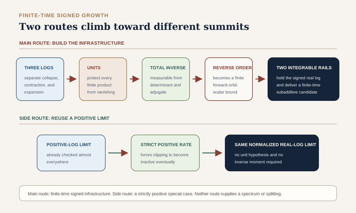
The diagram separates two logical products. The candidate theorem says that every finite slice is integrable and the process is shifted-subadditive. The positive-rate theorem says that one particular normalized sequence converges almost everywhere under probability and pre-ergodicity assumptions. Neither statement implies the other.
Motivation only: derivative cocycles in nonlinear dynamics
Let \(f:M\to M\) be a differentiable nonlinear map on a finite-dimensional manifold. A small tangent perturbation \(v\) at a state \(x\) is transported to first order by the derivative \(D f_x\). Repeated application suggests the ordered derivative product
\[ D f^n_x =D f_{f^{n-1}(x)}\cdots D f_{f(x)}D f_x. \]This is the standard motivating picture for a matrix cocycle. The orbit \(x,f(x),f^2(x),\ldots\) supplies the base dynamics, and each Jacobian matrix supplies one generator.
The forward norm asks how much the most amplified tangent direction can grow:
\[ \lVert D f^n_x v\rVert \le \lVert D f^n_x\rVert\lVert v\rVert. \]Its positive logarithm records bursts of expansion. That is useful for sensitivity, instability, and finite-time amplification, but it hides strong contraction.
When the derivative is invertible, the inverse norm probes the weakest forward direction. A large inverse norm means that some unit vector is mapped to a very small vector, or equivalently that recovering a perturbation from its image is poorly conditioned. In numerical language, the pair of forward and inverse norms separates amplification from near-collapse. In dynamical language, it distinguishes the most expanding direction from the strongest finite-time contraction visible to the chosen norm.
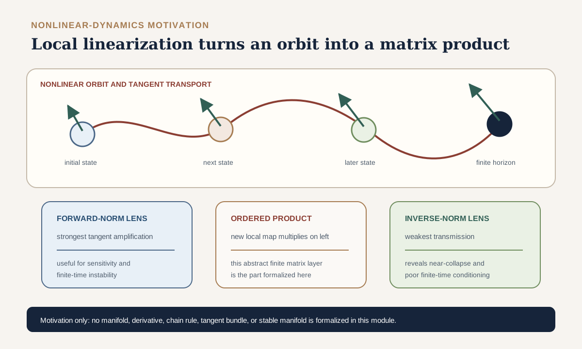
The finite-time sandwich is therefore a natural analytic prerequisite for later nonlinear work. It says that the signed log norm is not allowed to develop an uncontrolled negative tail when the inverse-generator positive log is integrable. It does not yet identify a physical Lyapunov exponent, a stable direction, or a tangent-space splitting.
Separate the three logarithms
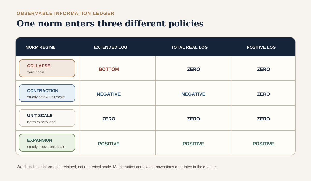
One input, three information policies
For a nonnegative scalar \(r\), the three observables behave as follows.
| Norm regime | Extended logarithm | Total real logarithm | Positive logarithm |
|---|---|---|---|
| \(r=0\) | \(\bot\) | \(0\) | \(0\) |
| \(0\lt r\lt1\) | \(\log r\lt0\) | \(\log r\lt0\) | \(0\) |
| \(r=1\) | \(0\) | \(0\) | \(0\) |
| \(r\gt1\) | \(\log r\gt0\) | \(\log r\gt0\) | \(\log r\gt0\) |
No column dominates the others in every role.
- The extended logarithm is zero-faithful. Exact collapse remains visible as bottom.
- The total real logarithm records finite contraction in an ordinary real codomain, but it erases exact collapse.
- The positive logarithm is a convenient nonnegative integrability envelope, but it erases every contraction as well as collapse.
In Lean: name the signed finite-time observable
C.realLogNormObservable k ωCis the bundled one-sided discrete matrix cocycle.k : ℕis the finite horizon, including \(0\).ωis the sample point in \(\Omega\).C.value k ωis the newest-factor-left finite product.‖...‖is the selected maximum row-sum operator norm.Real.logis total in Lean, soReal.log 0 = 0; this syntax does not make the observable zero-faithful.
The first four compiled boundary examples make this table executable:
\[ \operatorname{Real.log}0=0, \qquad \log^+(1/2)=0, \qquad \operatorname{Real.log}(1/2)\lt0, \qquad \log^+((1/2)^{-1})\gt0. \]The distinction matters immediately. If every generator contracts by one half, then \(P_n=0\) for every \(n\), while \(R_n=n\log(1/2)\) is strictly negative for positive \(n\). A theorem about \(P_n/n\) therefore cannot be narrated as a signed growth theorem.
Why measurability does not restore meaning
Both totalization choices are measurable. That is an analytic convenience, not a semantic guarantee. A singular matrix can satisfy
\[ \operatorname{Real.log}\lVert A\rVert=0 \]when \(A=0\), and its total inverse can satisfy
\[ \log^+\lVert A^{-1}\rVert=0. \]Those equalities do not say that collapse has zero strength. They say that the selected total functions return zero on the singular branch.
Propagate pointwise units
The algebraic hypothesis
RMT-34 defines
def IsPointwiseInvertible
    (C : DiscreteMatrixCocycle (ι := ι) μ) : Prop :=
  ∀ ω, IsUnit (C.generator ω)
This is a statement at every sample \(\omega\). It is not an almost-everywhere representative condition. It does not imply a uniform condition-number bound, an inverse moment, independence, or an invertible base map.
The identity value \(C_0\) is a unit. If \(C_n(\omega)\) is a unit and \(A(T^n\omega)\) is a unit, then their product is a unit. Induction proves
\[ \operatorname{IsUnit}(C_n(\omega)) \]for every natural \(n\) and every \(\omega\).
The nonempty bridge
In a nonempty matrix dimension, a unit matrix is nonzero and therefore has strictly positive norm. The extended and real logarithms then agree:
\[ L_n(\omega)=\bigl(R_n(\omega):\overline{\mathbb R}\bigr). \]The nonempty premise is essential. For matrices indexed by the empty type, the matrix ring has one element, so \(0=I\) and the zero matrix is a unit. The selected row-sum norm is still zero because there are no rows. Hence
\[ L_n(\omega)=\bot, \qquad R_n(\omega)=0. \]RMT-34 keeps the nonempty typeclass only on this bridge. Its real-valued subadditivity, lower rail, integrability theorem, and candidate remain valid in empty dimension through explicit zero branches.
Signed subadditivity
The cocycle law and norm submultiplicativity give
\[ \lVert C_{m+k}(\omega)\rVert \le \lVert C_k(T^m\omega)\rVert\lVert C_m(\omega)\rVert. \]Under pointwise units in nonempty dimension, both factors and their product have positive norm. Monotonicity of the logarithm and the logarithm product law yield
\[ R_{m+k}(\omega) \le R_k(T^m\omega)+R_m(\omega). \]The empty branch is identically zero.
In Lean: state signed shifted subadditivity
hC.realLogNormObservable_add_le m k ωhC : C.IsPointwiseInvertibleis the pointwise unit proof.mis the earlier block length andkis the shifted later block length.C.base^[m] ωis Lean’s notation for \(T^m\omega\).- The receiver dot in
hC.realLogNormObservable_add_lesupplies the unit hypothesis to the theorem namespace. - The conclusion is pointwise for every
ω, not merely almost everywhere. - No moment, probability, ergodicity, or nonempty-index hypothesis appears in this public real-valued statement.
This hypothesis is not cosmetic. Set
\[ A= \begin{bmatrix} 1/2&0\\ 0&0 \end{bmatrix}, \qquad B= \begin{bmatrix} 0&0\\ 0&1/2 \end{bmatrix}. \]Then \(\lVert A\rVert=\lVert B\rVert=1/2\), but \(AB=0\). Total real-log subadditivity would demand
\[ 0=\operatorname{Real.log}\lVert AB\rVert \le 2\operatorname{Real.log}(1/2)\lt0, \]which is false. The module compiles this exact counterexample.
Build a measurable total inverse
The obstacle
The generator \(A:\Omega\to\operatorname{Mat}_{\iota}(\mathbb C)\) is measurable entrywise. RMT-34 needs measurability of
\[ \omega\longmapsto\log^+\lVert A(\omega)^{-1}\rVert \]without placing invertibility in the measurability theorem’s signature. The pinned library does not expose a matrix-level measurable-inverse instance that closes this goal directly.
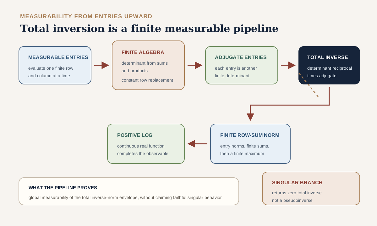
The finite construction
The module builds the proof from exact finite operations.
Expand the determinant as a finite sum over permutations of finite products of entries.
Prove that replacing one row by a constant row preserves entrywise measurability.
Express every adjugate entry, part of the transposed cofactor construction, as a determinant of a row-updated matrix.
Use Mathlib’s total inverse formula
\[ A^{-1}=\det(A)^{-1}\operatorname{adj}(A). \]Unfold the selected matrix norm as a finite supremum of finite row sums.
Compose with the continuous positive-log function.
In Lean: prove the total inverse envelope measurable
C.measurable_inverseGeneratorLogPlusNormObservableinverseGeneratorLogPlusNormObservableis \(\omega\mapsto\log^+\lVert A(\omega)^{-1}\rVert\).- The superscript-looking Lean inverse is implemented by Mathlib’s total nonsingular inverse.
measurable_...concludes ordinary measurability, not integrability.- The theorem uses the cocycle’s
measurable_generatorfield and the private determinant-adjugate support chain. - No unit hypothesis is required because the total inverse is defined as zero on the singular locus.
This yields unconditional measurability of \(G\) and every \(Q_n\). Pointwise units are introduced later, when these totalized functions are interpreted as genuine inverse norms.
Why private placement is appropriate
The determinant, row-update, adjugate, inverse, and matrix-norm measurability lemmas are private in this module. They are general enough to be candidates for a future random-matrix utility layer, but RMT-34 first needs them as a focused support chain. Keeping them private avoids freezing a generic public application programming interface (API) before that reuse has been tested.
Reverse inverse products in the correct order
Inversion changes chronological order
Matrix inversion obeys
\[ (AB)^{-1}=B^{-1}A^{-1}. \]Therefore
\[ C_n(\omega)^{-1} =A(\omega)^{-1}A(T\omega)^{-1}\cdots A(T^{n-1}\omega)^{-1}. \]The earliest inverse factor appears on the left. This is the reverse of the newest-factor-left forward product.
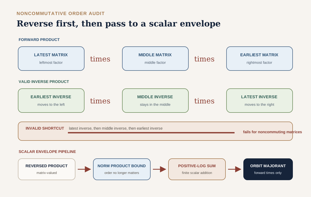
The compiled upper and lower shear example gives a counterexample to equality of the two inverse orders. This rules out the same-order inverse-cocycle formula.
The finite inverse orbit majorant
The finite inverse-value envelope is
\[ Q_n(\omega)=\log^+\lVert C_n(\omega)^{-1}\rVert. \]The forward-orbit inverse-generator sum is
\[ J_n(\omega) =\sum_{j=0}^{n-1} \log^+\lVert A(T^j\omega)^{-1}\rVert. \]It satisfies
\[ J_0=0 \]and
\[ J_{n+1}(\omega) =J_n(\omega)+G(T^n\omega). \]Induction, reverse-order inversion, norm submultiplicativity, monotonicity of positive log, and the positive-log product inequality prove
\[ Q_n(\omega)\le J_n(\omega). \]In Lean: compare the inverse value with its orbit envelope
C.inverseValueLogPlusNormObservable_le_inverseOrbitLogPlusSum k ωinverseValueLogPlusNormObservableis the left side \(Q_k\): first build the entire newest-factor-left product, then invert it.leis the order relation \(\le\).inverseOrbitLogPlusSumis the right side \(J_k\): a scalar sum over \(j=0,\ldots,k-1\).- The proof reverses matrix factors before taking norms. The scalar summands may then be written in increasing chronological base order because real addition is commutative.
kandωare literal theorem arguments; there is no hidden expectation or limit.- No unit hypothesis occurs in this call. Mathlib’s total inverse makes the statement defined even at singular matrices, but the singular branch then loses quantitative information about collapse.
This inequality is unconditional because total inversion and positive log are defined on singular matrices. On a singular input, however, \(Q_n\) may be zero. The inequality then carries no quantitative record of collapse.
Construct the two-rail sandwich
The lower rail for one value
Let \(M\) be a unit matrix in nonempty dimension. The selected operator norm is submultiplicative, so
\[ 1=\lVert I\rVert =\lVert M^{-1}M\rVert \le \lVert M^{-1}\rVert\lVert M\rVert. \]Taking logarithms gives
\[ 0 \le \log\lVert M^{-1}\rVert+\log\lVert M\rVert. \]Since
\[ \log\lVert M^{-1}\rVert \le \log^+\lVert M^{-1}\rVert, \]we obtain
\[ -\log^+\lVert M^{-1}\rVert \le \log\lVert M\rVert. \]Apply this to \(M=C_n(\omega)\), then use \(Q_n\le J_n\). Negation reverses the latter inequality:
\[ -J_n(\omega) \le -Q_n(\omega) \le R_n(\omega). \]The empty-dimensional branch is separately zero.
The upper rail
For every real number \(x\),
\[ x\le\max\{0,x\}. \]Therefore, without any invertibility assumption,
\[ R_n(\omega)\le P_n(\omega). \]Together the rails are
\[ -J_n(\omega) \le R_n(\omega) \le P_n(\omega). \]In Lean: place the signed observable between the rails
hC.neg_inverseOrbitLogPlusSum_le_realLogNormObservable k ωhC : C.IsPointwiseInvertiblesupplies the unit proof needed only for the lower comparison.neg_inverseOrbitLogPlusSummeans the unary minus applied to \(J_k\); Lean’s theorem name spells out that lower endpoint.realLogNormObservableis the signed middle \(R_k\).k ωspecialize a pointwise theorem at one finite horizon and sample.- The companion upper theorem is typed as
C.realLogNormObservable_le_logPlusNormObservable k ω; it requires no invertibility. - Neither comparison claims equality. The two-rate diagonal example below makes the lower inequality strict.
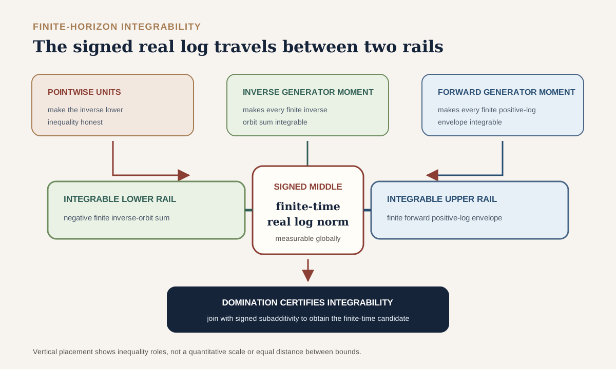
Make both rails integrable
The structure
structure HasIntegrableGeneratorLogTails
    (C : DiscreteMatrixCocycle (ι := ι) μ) : Prop where
  isPointwiseInvertible : C.IsPointwiseInvertible
  hasIntegrableGeneratorLogPlus : C.HasIntegrableGeneratorLogPlus
  integrable_inverseGeneratorLogPlus :
    Integrable C.inverseGeneratorLogPlusNormObservable μ
contains three distinct obligations.
| Field | What it licenses | What it does not license |
|---|---|---|
| Pointwise units | Genuine inverses, signed subadditivity, lower rail | Any moment bound |
| Forward positive-log integrability | Integrable upper rail \(P_n\) | Contraction control |
| Inverse positive-log integrability | Integrable lower rail \(-J_n\) | Negative time or an inverse exponent |
Measure preservation transports integrability of \(G\) through each nonnegative iterate \(T^j\). Finite-sum closure makes \(J_n\) integrable. Earlier work already makes \(P_n\) integrable from the forward generator moment. The real log \(R_n\) is measurable unconditionally. Mathlib’s two-sided domination theorem then proves
\[ \operatorname{Integrable}(R_n,\mu) \]for every natural \(n\).
In Lean: certify finite-horizon signed integrability
hC.integrable_realLogNormObservable k- Here
hC : C.HasIntegrableGeneratorLogTailsis the three-field package in the preceding code block. integrable_...means the absolute value has a finite integral with respect toμ; it is stronger than measurability.realLogNormObservable kis the function \(\omega\mapsto R_k(\omega)\), not a single sampled value.- The proof combines the measurable middle, the integrable lower and upper rails, and a two-sided domination theorem.
k : ℕis arbitrary but finite. This declaration does not assert integrability of a limit as \(k\to\infty\).
The lower inequality itself requires only pointwise units. RMT-34 exposes it
on the weaker receiver IsPointwiseInvertible, not on the full
three-field integrability package.
Package the signed process
An integrable shifted-subadditive process candidate records two fields:
- every finite slice is integrable;
- the shifted subadditive inequality holds pointwise.
The theorem
theorem HasIntegrableGeneratorLogTails.isIntegrableSubadditiveProcessCandidate
    (hC : C.HasIntegrableGeneratorLogTails) :
    IsIntegrableSubadditiveProcessCandidate C.base μ
      C.realLogNormObservable
fills those fields with the sandwich integrability theorem and the pointwise-unit subadditivity theorem.
In Lean: package exactly the input expected downstream
hC.isIntegrableSubadditiveProcessCandidate- The same
hC : C.HasIntegrableGeneratorLogTailsprovides both tail moments and pointwise units. isIntegrableSubadditiveProcessCandidatereturns a structure-valued proof; it does not run an ergodic theorem.- Its integrability field is filled by
hC.integrable_realLogNormObservable. - Its shifted-subadditivity field is filled by
hC.isPointwiseInvertible.realLogNormObservable_add_le. - There is no horizon argument because this one proof packages the entire family \(k\mapsto R_k\).
This candidate is infrastructure, not convergence. RMT-34 does not define a signed integrated Fekete rate, rerun the lower-deviation machinery for this new process, or prove that \(R_n/n\) converges in general.
Test the missing inverse tail
The infinite-Lebesgue boundary
The simplest separation uses a constant contraction by one half on the real line with Lebesgue measure. Its forward positive log is zero:
\[ \log^+(1/2)=0. \]Its inverse positive log is the nonzero constant
\[ \log^+((1/2)^{-1})=\log 2. \]The zero function is integrable on every measure space. A nonzero constant is not integrable over the whole real line because Lebesgue measure has infinite total mass. The module contains formal proofs of
\[ \operatorname{Integrable}(0,\operatorname{volume}) \]and
\[ \neg\operatorname{Integrable}(\log 2,\operatorname{volume}). \]This boundary is distinct from the probability example below. On a probability space every finite constant is integrable, so a constant cannot separate the two moment conditions.
A geometric probability law
Mathlib’s geometric measure with parameter \(p\) assigns mass
\[ (1-p)^n p \]to \(n\in\mathbb N\), when \(p\ne0\). RMT-34 fixes \(p=1/2\), hence
\[ \mathbb P\{N=n\}=2^{-(n+1)}. \]At atom \(n\), define the one-dimensional complex matrix
\[ A(n)= \begin{bmatrix} \exp(-2^n) \end{bmatrix}. \]It is a unit, and the selected norm and inverse norm are
\[ \lVert A(n)\rVert=\exp(-2^n), \qquad \lVert A(n)^{-1}\rVert=\exp(2^n). \]Therefore
\[ \begin{aligned} \log^+\lVert A(n)\rVert&=0,\\ \log^+\lVert A(n)^{-1}\rVert&=2^n,\\ \operatorname{Real.log}\lVert A(n)\rVert&=-2^n. \end{aligned} \]The absolute inverse and signed tails have the same weighted term:
\[ 2^{-(n+1)}2^n=\frac12. \]The series of constant one-half terms diverges. Mathlib’s exact
integrable_geometricMeasure_iff theorem converts that divergence
into failure of integrability for both missing tails. The forward
positive-log observable is identically zero and therefore integrable.
The final compiled conjunction checks all five claims together:
- the geometric measure is a probability measure;
- every one-dimensional generator is a unit;
- the forward generator positive-log hypothesis holds;
- the inverse-generator positive log is not integrable;
- the one-step signed real log is not integrable.
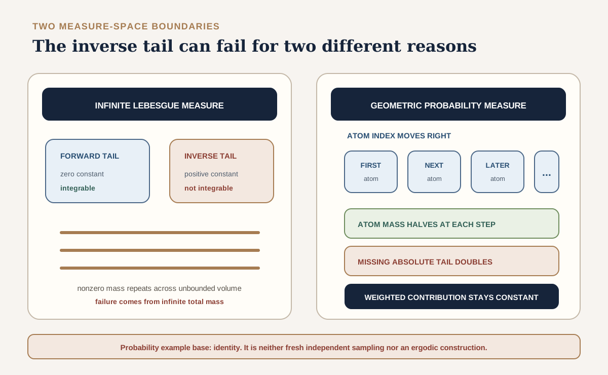
This is not independent sampling and not an ergodic construction
The cocycle’s base map is exactly id. Once an atom \(n\) is
selected, every forward base iterate remains at that same atom. The example
is therefore not an independent and identically distributed sequence of fresh
draws.
It is also not an ergodic base construction. The singleton containing atom zero is invariant under the identity map and has probability one half. This elementary nonergodicity observation is not needed by the compiled five-part conjunction. The Lean-checked purpose of the example is one-step moment separation on a genuine probability space.
The conclusion is one-way and precise:
Forward positive-log integrability does not imply inverse-generator positive-log integrability or one-step signed real-log integrability, even when every generator is an invertible one-dimensional matrix.
The module does not compile the reciprocal example, so this chapter does not claim that the two moment conditions are logically independent in both directions.
Use strict positive rate
Begin with the RMT-33 limit
Assume now that \(\mu\) is a probability measure, the base is pre-ergodic, and the forward generator positive log is integrable. Here pre-ergodic means that invariant measurable sets satisfy the ergodic zero-or-full rigidity condition, without separately bundling measure preservation. The cocycle already stores preservation. RMT-33 gives
\[ \frac{P_n(\omega)}{n} \longrightarrow \gamma_+(C) \]for almost every \(\omega\), where \(\gamma_+(C)\) is the integrated positive-log growth rate.
Add the strict hypothesis
\[ 0\lt\gamma_+(C). \]For a sample where the convergence holds, the normalized value is eventually larger than \(\gamma_+(C)/2\), which is positive. At every such horizon \(n\ge1\), positivity of \(P_n(\omega)/n\) forces \(P_n(\omega)\gt0\).
By definition,
\[ P_n(\omega)=\max\{0,R_n(\omega)\}. \]If that maximum is positive, its real-log branch is positive and
\[ P_n(\omega)=R_n(\omega). \]The normalized positive-log and real-log sequences are eventually equal. Eventual equality transfers convergence:
\[ \frac{R_n(\omega)}{n} \longrightarrow \gamma_+(C) \]for almost every \(\omega\).
In Lean: transfer the limit on the strictly positive branch
hC.ae_tendsto_normalizedRealLogNormObservable_of_pos hT hpos- Here
hC : C.HasIntegrableGeneratorLogPlusis only the forward positive-log integrability package; this shortcut does not consume the two-tail package. hT : PreErgodic C.base μsupplies the invariant-set rigidity used by the preceding RMT-33 convergence theorem. Preservation is already stored inC.hpos : 0 < C.integratedLogPlusGrowthRate hCis the literal strict branch-selection hypothesis; the rate consumes the forward-integrability witnesshC, not the measure as an explicit final argument.ae_tendstomeans convergence for \(\mu\)-almost every sample; it is not a pointwise-for-all-samples claim.- The theorem’s conclusion writes
(fun n ↦ normalizedProcess C.realLogNormObservable n ω). HerenormalizedProcessdivides the signed observable by the horizon using the repository’s total convention at \(n=0\); there is no separate declaration namednormalizedRealLogNormObservable. - No unit or inverse-tail argument appears because eventual positivity turns off clipping directly.
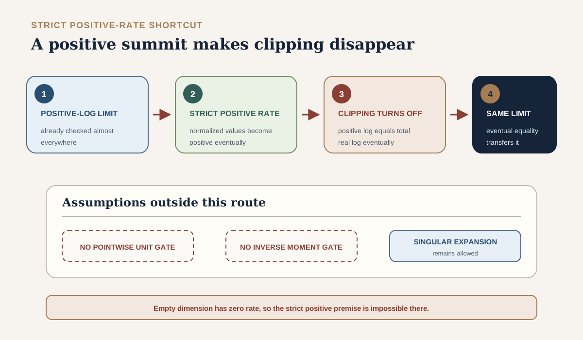
Why invertibility is absent
A singular matrix can still have expanding top norm. The compiled matrix
\[ \begin{bmatrix} 2&0\\ 0&0 \end{bmatrix} \]is singular and has selected norm two. Positive growth can therefore live on a singular range. Requiring units in the shortcut theorem would discard a valid regime without helping the proof.
Why empty dimension is only vacuous
In empty dimension every log-positive observable is zero. The module compiles the identity
\[ \gamma_+(C)=0 \]for every empty-dimensional cocycle satisfying the forward integrability package. The theorem’s strict positivity premise cannot be supplied there. The signature remains dimension-uniform, but its empty specialization has no substantive instance.
Why zero rate is not enough
For the constant scalar contraction \(A=1/2\),
\[ \frac{P_n}{n}=0 \]and
\[ \frac{R_n}{n}=\log(1/2)\lt0. \]Thus a nonnegative limiting rate, or even a zero rate, does not force eventual agreement. Strict positivity is the exact branch-selection mechanism used by the proof.
Read the boundary atlas
Each compiled model rejects a different overclaim.
| Boundary | Checked fact | Claim it blocks |
|---|---|---|
| Real zero | \(\operatorname{Real.log}0=0\) | Total real log is zero-faithful |
| Scalar contraction | Positive log is zero, signed log is negative | Positive log records contraction |
| Empty matrix index | Zero matrix is a unit, extended log is bottom, real log is zero | Units alone imply the extended-to-real bridge without nonempty dimension |
| Singular contractions | Two norm-one-half factors multiply to zero | Total real log is subadditive without nonvanishing |
| Singular inverse | Total nonsingular inverse is zero | Inverse envelope measures collapse on singular matrices |
| Noncommuting shears | Same-order and reverse-order inverse products differ | A same-order inverse product is the forward product’s inverse |
| Two-rate contraction | Inverse norm sees the strongest contraction | Inverse envelope equals the negative top log norm |
| Infinite Lebesgue measure | A positive constant can be nonintegrable | Constant moments behave as on probability spaces |
| Geometric probability law | Forward moment holds while inverse and signed moments fail | Forward moment implies the missing inverse moment |
| Singular expansion | A singular matrix has norm greater than one | Positive-rate transfer needs units |
| Empty positive rate | Integrated positive-log rate is zero | Strict positive rate has a substantive empty-dimensional case |
For the two-rate matrix
\[ D= \begin{bmatrix} 1/2&0\\ 0&1/4 \end{bmatrix}, \]the selected norm is \(1/2\), while \(\lVert D^{-1}\rVert=4\). Hence
\[ -\log^+\lVert D^{-1}\rVert =-\log4 \lt -\log2 =\log\lVert D\rVert. \]The lower rail is genuinely a bound, not an identity.
Audit the complete checked surface
The source audited for this chapter is exactly the 942-line file with the
Secure Hash Algorithm 256-bit (SHA-256) digest
ac950f8728e5fd003cff3b7a5d0750e5c36060730b3ebadc5b0e1165b54e72ea.
If that hash changes, the declaration and line ledgers must be regenerated.
Public declaration ledger
| Number | Public declaration | Exact job | Essential gate |
|---|---|---|---|
| 1 | realLogNormObservable | Define \(R_n\) | Total real logarithm |
| 2 | IsPointwiseInvertible | Require every generator to be a unit | Pointwise, not almost everywhere |
| 3 | IsPointwiseInvertible.value_isUnit | Propagate units to every finite value | Newest-factor-left induction |
| 4 | IsPointwiseInvertible.logNormObservable_eq_coe_realLogNormObservable | Bridge extended and real logs | Nonempty index and units |
| 5 | measurable_realLogNormObservable | Prove \(R_n\) measurable | No units required |
| 6 | realLogNormObservable_eq_zero_of_isEmpty | Identify the empty-dimensional real observable | Empty index |
| 7 | realLogNormObservable_zero | Prove \(R_0=0\) in every finite dimension | Empty/nonempty split |
| 8 | realLogNormObservable_one | Rewrite \(R_1\) as generator real log norm | Cocycle time-one identity |
| 9 | IsPointwiseInvertible.realLogNormObservable_add_le | Prove signed shifted subadditivity | Units, with explicit empty branch |
| 10 | inverseGeneratorLogPlusNormObservable | Define \(G\) | Total nonsingular inverse |
| 11 | measurable_inverseGeneratorLogPlusNormObservable | Prove \(G\) measurable | Determinant-adjugate pipeline |
| 12 | inverseValueLogPlusNormObservable | Define \(Q_n\) | Total finite-value inverse |
| 13 | inverseValueLogPlusNormObservable_zero | Prove \(Q_0=0\) | Empty/nonempty split |
| 14 | inverseValueLogPlusNormObservable_one | Identify \(Q_1=G\) | Cocycle time-one identity |
| 15 | measurable_inverseValueLogPlusNormObservable | Prove every \(Q_n\) measurable | Total inverse measurability |
| 16 | inverseOrbitLogPlusSum | Define \(J_n\) | Forward base iterates only |
| 17 | inverseOrbitLogPlusSum_zero | Prove \(J_0=0\) | Empty finite range |
| 18 | inverseOrbitLogPlusSum_succ | Append the newest inverse term | Finite sum recurrence |
| 19 | inverseValueLogPlusNormObservable_le_inverseOrbitLogPlusSum | Prove \(Q_n\le J_n\) | Reverse-order inverse and positive-log product bound |
| 20 | HasIntegrableGeneratorLogTails | Package units and the two generator moments | Three separate fields |
| 21 | measurable_inverseOrbitLogPlusSum | Prove \(J_n\) measurable | Measurable iterates and finite sums |
| 22 | HasIntegrableGeneratorLogTails.integrable_inverseGeneratorLogPlus_at_base_iterate | Transport inverse-tail integrability through \(T^j\) | Measure preservation |
| 23 | HasIntegrableGeneratorLogTails.integrable_inverseOrbitLogPlusSum | Prove \(J_n\) integrable | Finite sum of transported terms |
| 24 | IsPointwiseInvertible.neg_inverseOrbitLogPlusSum_le_realLogNormObservable | Prove \(-J_n\le R_n\) | Units only |
| 25 | realLogNormObservable_le_logPlusNormObservable | Prove \(R_n\le P_n\) | Unconditional max inequality |
| 26 | HasIntegrableGeneratorLogTails.integrable_realLogNormObservable | Prove every \(R_n\) integrable | Measurability plus two integrable rails |
| 27 | HasIntegrableGeneratorLogTails.isIntegrableSubadditiveProcessCandidate | Package the signed finite-time candidate | Declarations 9 and 26 |
| 28 | HasIntegrableGeneratorLogPlus.ae_tendsto_normalizedRealLogNormObservable_of_pos | Transfer RMT-33 convergence to \(R_n/n\) | Probability, pre-ergodicity, and strict positive rate |
The public surface deliberately separates total measurability from faithful inverse interpretation. Declarations 5, 11, 15, 19, 21, and 25 require no unit hypothesis. Declarations 3, 4, 9, and 24 expose the algebraic gates that make the signed interpretation valid.
Private support ledger
| Source line | Private item | Exact job |
|---|---|---|
| 198 | measurable_matrixDet | Expand determinant into measurable finite sums and products |
| 211 | measurable_updateRow_const | Preserve entrywise measurability under a constant row replacement |
| 224 | measurable_matrixAdjugate | Reduce adjugate entries to row-update determinants |
| 234 | measurable_matrixInverse | Apply the total determinant-adjugate inverse formula |
| 249 | measurable_matrixNorm | Unfold the selected row-sum norm as finite measurable operations |
| 437 | neg_inverseValueLogPlus_le_realLogNorm | Prove the nonempty one-value lower rail |
| 638 | singularExpandingMatrix | Store the singular expansion boundary |
| 673 | geometricTailParameter | Fix the geometric parameter at one half |
| 676 | geometricTailMeasure | Define the geometric probability measure |
| 679 | unnamed private instance | Register the probability-measure instance |
| 683 | geometricTailExponent | Define the tail size \(2^n\) |
| 686 | geometricTailMatrix | Define the scalar contraction \(\exp(-2^n)\) |
| 689 | geometricTailCocycle | Bundle identity base, generator, preservation, and measurability |
| 696 | geometricTailParameter_ne_zero | Discharge the geometric theorem’s nonzero parameter gate |
| 702 | geometricTailMatrix_norm | Compute the forward norm |
| 708 | geometricTailMatrix_inv | Compute the scalar matrix inverse |
| 717 | geometricTailMatrix_inv_norm | Compute the inverse norm |
| 722 | geometricTailCocycle_isPointwiseInvertible | Prove every geometric-tail generator is a unit |
| 728 | geometricTail_forward_logPlus | Compute the forward positive log as zero |
| 735 | geometricTail_inverse_logPlus | Compute the inverse positive log as \(2^n\) |
| 743 | geometricTail_realLog | Compute the signed real log as \(-2^n\) |
| 747 | geometricTail_forward_observable | Lift the scalar forward identity to the cocycle |
| 755 | geometricTail_inverse_observable | Identify the inverse observable with the exponent function |
| 764 | geometricTail_real_observable | Identify the one-step signed observable |
| 773 | geometricTail_not_summable | Reduce every weighted absolute term to one half |
| 792 | geometricTail_hasIntegrableGeneratorLogPlus | Prove the zero forward observable integrable |
| 797 | geometricTail_not_integrable_inverse | Convert nonsummability into inverse-tail nonintegrability |
| 805 | geometricTail_not_integrable_real | Convert nonsummability into signed nonintegrability |
| 833 | singularFirstContraction | Store the first singular subadditivity factor |
| 836 | singularSecondContraction | Store the second factor whose product vanishes |
| 876 | twoRateContraction | Store the two-rate diagonal contraction |
| 879 | twoRateInverse | Store its explicit inverse |
| 914 | upperShear | Store one noncommuting unit shear |
| 917 | lowerShear | Store the other noncommuting unit shear |
The first five private items are measurability infrastructure, and the sixth is lower-rail proof infrastructure. The remaining private items are compiled semantic fixtures and tests. Private placement does not make their mathematics informal; it prevents boundary fixtures from becoming library API.
Exact source-order map
| Source span | Contents |
|---|---|
| Lines 73 to 193 | Public declarations 1 to 10 |
| Lines 198 to 267 | Five private measurability helpers |
| Lines 271 to 433 | Public declarations 11 to 23 |
| Lines 437 to 462 | Private one-value lower lemma |
| Lines 467 to 577 | Public declarations 24 to 28 |
| Lines 581 to 636 | Compiled examples 1 to 9 |
| Lines 638 to 647 | Singular-expansion fixture and example 10 |
| Lines 654 to 671 | Infinite-measure example 11 |
| Lines 673 to 811 | Geometric probability construction |
| Lines 813 to 831 | Probability certificate comments and compiled example 12 |
| Lines 833 to 874 | Singular-contraction fixtures and examples 13 and 14 |
| Lines 876 to 912 | Two-rate fixtures and example 15 |
| Lines 914 to 928 | Shear fixtures and example 16 |
| Lines 932 to 942 | Eleven axiom prints |
Assumption ledger
| Assumption | First use | What it licenses | What it does not license |
|---|---|---|---|
| Finite index type | Matrix and determinant setup | Finite determinants, adjugates, row sums, and products | Nonempty dimension |
| Decidable equality on the index | Matrix updates and finite combinatorics | Entrywise constructions | Analytic bounds |
| Measurable space on \(\Omega\) | Ambient cocycle setup | Measurable observables and integrals | Probability normalization |
| Generator measurability | Cocycle field | Measurability of values and inverse envelopes | Invertibility |
| Base measure preservation | Cocycle field | Measurable iterates and transport of integrability | Ergodicity or invertible base |
| Pointwise generator units | IsPointwiseInvertible | Unit finite values, signed subadditivity, genuine inverse lower rail | Integrability, uniform conditioning, or almost-everywhere relaxation |
| Nonempty index | Extended-to-real bridge and private one-value proof | Positive norm for nonzero unit matrices | Needed by the final real-valued package |
| Forward generator positive-log integrability | Tail package and shortcut | Integrable \(P_n\) and the RMT-33 input | Inverse-tail or signed integrability |
| Inverse generator positive-log integrability | Tail package | Integrable \(J_n\) | Negative-time dynamics or an inverse exponent |
| Probability measure | Geometric example and shortcut | Unit total mass and RMT-33 probability endpoint | Independence or ergodicity |
| Pre-ergodicity | Positive-rate shortcut | Combines with bundled preservation for RMT-33 | Any finite-time sandwich step |
| Strict positive integrated rate | Positive-rate shortcut | Eventual removal of clipping | A conclusion at zero or negative rate |
Pinned Mathlib API ledger
The repository pins Lean and Mathlib tag v4.32.0. The Mathlib
checkout is commit
81a5d257c8e410db227a6665ed08f64fea08e997.
| Pinned declaration | Role |
|---|---|
Matrix.det_apply | Determinant as a finite permutation sum |
Matrix.adjugate_apply | Adjugate entry through row replacement |
Matrix.inv_def | Total inverse as determinant reciprocal times adjugate |
Matrix.mul_inv_rev | Reverse inverse-product order |
Matrix.nonsing_inv_mul | Recover identity under a determinant unit |
Matrix.linfty_opNorm_def | Expose the selected maximum row-sum norm |
Real.posLog_mul | Additively majorize positive log of a product |
Real.posLog_le_posLog | Transport a nonnegative norm inequality |
Real.log_mul | Split a product logarithm under nonzero gates |
MeasurePreserving.integrable_comp_of_integrable | Transport an integrable function through a base iterate |
MeasureTheory.integrable_of_le_of_le | Certify the signed middle from two integrable rails |
ProbabilityTheory.geometricMeasure | Define the atomic probability law |
integrable_geometricMeasure_iff | Convert geometric-law integrability to weighted summability |
Filter.Tendsto.congr’ | Transfer convergence under eventual equality |
Compiled example ledger
- Total real log sends zero to zero.
- Positive log erases scalar contraction.
- Total real log records scalar contraction.
- Inverse positive log records the missing scalar tail.
- The empty-dimensional zero matrix is a unit.
- Every empty-dimensional cocycle is pointwise invertible.
- Empty dimension separates extended bottom from real zero.
- Empty dimension has zero integrated positive-log rate.
- Matrix inversion reverses two-factor order.
- A singular matrix can have norm greater than one.
- Infinite Lebesgue measure separates zero and nonzero constants.
- The geometric probability cocycle separates forward from inverse and signed moments.
- Total real-log subadditivity fails for singular factors with zero product.
- The total-inverse lower rail fails on a singular contraction.
- A two-rate contraction makes the lower rail strict.
- Noncommuting shears separate same-order and reverse-order inverse products.
Axiom surface
The source prints axioms for these eleven public theorems, in this exact source order:
IsPointwiseInvertible.value_isUnitIsPointwiseInvertible.logNormObservable_eq_coe_realLogNormObservablemeasurable_realLogNormObservableIsPointwiseInvertible.realLogNormObservable_add_lemeasurable_inverseGeneratorLogPlusNormObservableinverseValueLogPlusNormObservable_le_inverseOrbitLogPlusSumHasIntegrableGeneratorLogTails.integrable_inverseOrbitLogPlusSumIsPointwiseInvertible.neg_inverseOrbitLogPlusSum_le_realLogNormObservableHasIntegrableGeneratorLogTails.integrable_realLogNormObservableHasIntegrableGeneratorLogTails.isIntegrableSubadditiveProcessCandidateHasIntegrableGeneratorLogPlus.ae_tendsto_normalizedRealLogNormObservable_of_pos
Every print reports exactly
propext;Classical.choice; andQuot.sound.
There is no sorryAx, project-specific axiom, unsafe declaration,
sorry, or admit in the module.
The complete surface audit therefore records 28 public declaration commands,
three fields on HasIntegrableGeneratorLogTails, 34 private
commands, 16 compiled anonymous examples, and 11 explicit axiom prints. These
counts describe the frozen 942-line source, not a hand-selected theorem list.
Checked nonclaim ledger
RMT-34 does not prove any of the following:
- a general almost-everywhere limit for \(R_n/n\);
- a signed Kingman theorem for arbitrary integrable real subadditive processes;
- convergence in \(L^1\), convergence in probability as a separate theorem, or uniform convergence;
- interchange of a samplewise limit and an integral;
- an integrated signed Fekete rate;
- an equality between \(J_n\) and \(Q_n\);
- a same-base inverse cocycle;
- an invertible base map or a negative-time process;
- that a pointwise unit hypothesis follows from an almost-everywhere unit hypothesis without representative work;
- an identity between inverse-norm growth and the negative top exponent;
- singular-value limits, all Lyapunov exponents, or multiplicities;
- an invariant filtration or splitting;
- an Oseledets multiplicative ergodic theorem;
- stable or unstable manifolds;
- a manifold, derivative, Jacobian, chain rule, tangent bundle, or derivative cocycle;
- independence, identical distribution, mixing, or a Markov property;
- an ergodic interpretation of the geometric identity-base example;
- a reciprocal counterexample proving both directions of logical independence between the two tail moments;
- a pseudoinverse or a quantitative measure of singular collapse;
- a rate of convergence, concentration inequality, or finite-sample confidence statement;
- a substantive positive-rate result in empty dimension.
Place the construction classically
The following primary sources explain why the forward moment, inverse moment, signed logarithm, and eventual spectrum should be kept distinct. They provide historical placement, not imported proof for the Lean declarations.
Furstenberg and Kesten, 1960
H. Furstenberg and H. Kesten’s “Products of Random Matrices” appeared in The Annals of Mathematical Statistics 31, pp. 457 to 469. The Hebrew University bibliographic record confirms the authors, journal, year, pages, and digital object identifier (DOI).
This paper is a foundational historical source for asymptotic random matrix products. This chapter does not assign it an unchecked theorem number or claim that the RMT-34 finite-time package reproduces its hypotheses.
Kingman, 1968
J. F. C. Kingman’s “The Ergodic Theory of Subadditive Stochastic Processes” appeared in Journal of the Royal Statistical Society, Series B 30(3), pp. 499 to 510, with DOI 10.1111/j.2517-6161.1968.tb00749.x. It is the primary historical source for the general subadditive stochastic-process ergodic theory that motivates the repository’s longer sequence.
RMT-34 only constructs a signed integrable subadditive candidate, plus one strictly positive-rate corollary from the already-checked log-positive theorem. It does not formalize Kingman’s full signed theorem here.
Oseledets, 1968
V. I. Oseledets’ original multiplicative ergodic theorem appeared in Trudy Moskovskogo Matematicheskogo Obshchestva 19, pp. 179 to 210; the English translation appeared in Transactions of the Moscow Mathematical Society 19, pp. 197 to 231.
Oseledets is a destination on the project’s mathematical horizon. The present module proves no spectrum, multiplicity statement, invariant filtration, or splitting, so the source is cited for placement rather than as a description of the checked endpoint.
Ruelle, 1979
David Ruelle’s “Ergodic Theory of Differentiable Dynamical Systems” appeared in Publications Mathématiques de l’IHÉS 50, pp. 27 to 58, with DOI 10.1007/BF02684768. The author-hosted scan provides the primary text.
Section 1, especially Theorem 1.1 and Corollary 1.2 on printed pp. 29 to 30, uses a forward positive-log norm condition in a subadditive matrix-product setting. Theorem 1.6 develops a forward filtration in which the lowest exponent may be negative infinity. Section 3, especially Theorem 3.1 on printed p. 35, moves to an invertible base and invertible matrices with both forward and inverse positive-log conditions, obtaining finite exponents and a splitting.
That contrast motivates RMT-34’s explicit separation of algebraic units, forward moments, and inverse moments. RMT-34 does not reproduce Ruelle’s Theorem 1.1, Corollary 1.2, Theorem 1.6, or Theorem 3.1, and it does not inherit their conclusions merely by using similar moment language.
What this ascent teaches
- Totality and semantic fidelity are different goals. A total function can be measurable everywhere while erasing the boundary phenomenon of interest.
- Algebraic and analytic hypotheses should be separate fields. Units validate signed identities; moments validate integration.
- Noncommutative order survives until norms remove it. Reverse the product first, then bound it.
- A finite orbit majorant need not be a cocycle. The scalar sum \(J_n\) is useful precisely because it avoids a false backward-dynamics formula.
- Two-sided domination is a finite-time bridge. It proves integrability of each signed slice without proving asymptotic convergence.
- One counterexample can close only one implication. The geometric example shows that the forward moment does not force the inverse moment; it does not by itself prove bilateral logical independence.
- Strict positivity can simplify totalized branches. Once the limit is positive, clipping is eventually inactive and a narrower theorem becomes available without inverse moments.
- Degenerate dimensions test interfaces. Empty matrices separate algebraic units from positive norm and keep vacuous endpoints visible.
Forty fully worked exercises
The exercises are arranged as eight ropes of five. Each solution is included so that the chapter can be used for self-study or as a seminar handout.
Rope I: three observables
Exercise 1: classify four scalar regimes
For \(r=0\), \(r=1/2\), \(r=1\), and \(r=2\), compute the extended logarithm, total real logarithm, and positive logarithm qualitatively as bottom, negative, zero, or positive.
Solution.
At \(r=0\), the extended logarithm is bottom, while both real-valued totalizations return zero. At \(r=1/2\), the ordinary logarithm is negative, so the extended and total real logarithms are negative and positive log clips the value to zero. At \(r=1\), every logarithm is zero. At \(r=2\), the ordinary logarithm is positive, so all three finite branches agree with \(\log2\).
The key split is not merely finite versus infinite. Positive log also changes finite negative values, while total real log changes only the zero input.
Exercise 2: compute a constant contraction
Let the scalar generator be \(A(\omega)=1/2\) on every sample and let the base be arbitrary. Compute \(C_n\), \(R_n\), and \(P_n\).
Solution.
Every factor is the same scalar, so
\[ C_n=(1/2)^n. \]For positive \(n\),
\[ R_n=\log((1/2)^n)=n\log(1/2). \]This is strictly negative. Since \((1/2)^n\le1\), positive log clips it:
\[ P_n=\log^+((1/2)^n)=0. \]At \(n=0\), \(C_0=1\) and both real-valued observables are zero. Therefore \(R_n/n=\log(1/2)\) at positive times, while \(P_n/n=0\). This is the smallest model showing that expansion-only convergence is not signed convergence.
Exercise 3: compute a constant expansion
Repeat Exercise 2 with scalar generator \(A(\omega)=2\).
Solution.
Now
\[ C_n=2^n. \]For positive \(n\),
\[ R_n=\log(2^n)=n\log2. \]The logarithm is already positive, so clipping does nothing:
\[ P_n=\log^+(2^n)=n\log2. \]Thus both normalized processes equal \(\log2\) at every positive horizon. This is the model behind the positive-rate shortcut: eventual expansion puts the sequence permanently in the branch where the two real observables agree.
Exercise 4: explain why real-log measurability needs no units
Why can \(R_n(\omega)=\operatorname{Real.log}\lVert C_n(\omega)\rVert\) be measurable even when \(C_n(\omega)\) is singular or zero?
Solution.
The finite-time matrix value is measurable, and the selected matrix norm is a measurable nonnegative real function. Mathlib’s total real logarithm is a measurable function on all of \(\mathbb R\), including zero. Composition therefore proves measurability without excluding singular values.
Units are needed for a different reason. They make the norm positive so that ordinary logarithm laws, such as the product law used in signed subadditivity, express their intended mathematics. Measurability asks whether preimages of measurable sets behave correctly; it does not ask whether zero has retained collapse information.
Exercise 5: audit empty dimension
Why can the unique matrix on the empty index type be both zero and a unit? What values do the extended and total real log norms take?
Solution.
A matrix indexed by the empty type has no entries, so there is only one such matrix. Consequently its zero and identity elements are equal. The identity is a unit, so the same unique matrix is a unit even when written as zero.
The selected row-sum norm takes a supremum over no rows and equals zero. Therefore the zero-faithful extended logarithm is bottom, while Lean’s total real logarithm is
\[ \operatorname{Real.log}0=0. \]This is why the extended-to-real bridge requires a nonempty index even though the real-valued package can retain an explicit all-zero empty branch.
Rope II: units and signed subadditivity
Exercise 6: propagate units by induction
Assume every \(A(\omega)\) is a unit. Prove that every \(C_n(\omega)\) is a unit.
Solution.
At \(n=0\), \(C_0(\omega)=I\), and the identity is a unit. Suppose \(C_n(\omega)\) is a unit. The successor recurrence is
\[ C_{n+1}(\omega)=A(T^n\omega)C_n(\omega). \]The first factor is a unit by the pointwise generator hypothesis, and the second factor is a unit by the induction hypothesis. Products of units are units. Induction closes the statement for every natural \(n\).
Notice that the proof uses only forward iterates \(T^n\). No inverse of \(T\) is constructed or required.
Exercise 7: derive signed subadditivity
Assume nonempty dimension and pointwise units. Derive
\[ R_{m+k}(\omega) \le R_k(T^m\omega)+R_m(\omega). \]Solution.
The cocycle law gives
\[ C_{m+k}(\omega)=C_k(T^m\omega)C_m(\omega). \]Norm submultiplicativity yields
\[ \lVert C_{m+k}(\omega)\rVert \le \lVert C_k(T^m\omega)\rVert \lVert C_m(\omega)\rVert. \]All three matrix values are units, hence nonzero. In nonempty dimension their norms are strictly positive. The real logarithm is monotone on positive inputs, and its product law is valid for the two nonzero norm factors. Applying those facts gives the required sum. The empty branch is handled separately by reducing every observable to zero.
Exercise 8: verify the singular counterexample
For
\[ A= \begin{bmatrix} 1/2&0\\ 0&0 \end{bmatrix}, \qquad B= \begin{bmatrix} 0&0\\ 0&1/2 \end{bmatrix}, \]show that total real-log subadditivity fails.
Solution.
Each matrix has maximum absolute row sum \(1/2\), so
\[ \log\lVert A\rVert+\log\lVert B\rVert =2\log(1/2)\lt0. \]Their product is zero because the nonzero diagonal positions do not align:
\[ AB=0. \]Lean’s total real logarithm sends its norm to zero:
\[ \operatorname{Real.log}\lVert AB\rVert =\operatorname{Real.log}0 =0. \]The desired inequality would be \(0\le2\log(1/2)\), which is false. This counterexample isolates nonvanishing as a semantic requirement for signed subadditivity.
Exercise 9: compare pointwise and almost-everywhere units
Why does an almost-everywhere unit hypothesis not directly fill the
pointwise add_le field of the candidate structure?
Solution.
The candidate’s shifted-subadditivity field is a statement for every \(\omega\), every \(m\), and every \(k\). An almost-everywhere hypothesis allows an exceptional null set where a generator may be singular. Products whose orbit visits that set can invalidate the pointwise logarithm laws used in the proof.
One could design an almost-everywhere process interface, choose measurable representatives, and prove that a common invariant exceptional set is harmless. RMT-34 does not do that work. Its pointwise unit definition matches the pointwise candidate field exactly.
Exercise 10: locate the nonempty assumption
Which parts of the main route genuinely require a nonempty matrix index, and which final public interfaces avoid it?
Solution.
The extended-to-real bridge genuinely requires nonempty dimension because a unit must then have positive norm. The private one-value inverse lower-bound argument also uses \(\lVert I\rVert=1\), which is a nonempty-dimensional fact for the selected norm.
The public real-valued subadditivity theorem, inverse-orbit lower rail, finite-time integrability theorem, and signed candidate split on whether the index is empty. Their empty branches are all zero, so their signatures need no nonempty typeclass. The positive-rate shortcut also omits nonempty dimension, but its strict premise is impossible in the empty case.
Rope III: measurable total inversion
Exercise 11: expand determinant measurability
Explain why the determinant of a measurable finite complex matrix family is measurable.
Solution.
For a finite index type, the determinant is a finite sum over permutations. Each summand is a sign multiplied by a finite product of selected matrix entries. Entry evaluation is measurable by the matrix family’s entrywise measurability. Finite products of measurable complex functions are measurable, constant scalar multiplication preserves measurability, and finite sums preserve measurability.
The argument is constructive at the level of the Leibniz formula. It does not need a general continuity theorem for determinant, although such a theorem would express the same finite-dimensional fact.
Exercise 12: reach the adjugate through row updates
Why does measurability of constant row updates help prove measurability of the adjugate?
Solution.
Mathlib expresses an adjugate entry as the determinant of a matrix obtained by replacing one row with a fixed basis row. For each entry, split on whether the queried row is the replaced row. On that row the entry is constant; off that row it is inherited from the original measurable matrix family. Thus the updated matrix remains measurable entrywise.
Exercise 11 then makes the determinant of each updated matrix measurable. Since every adjugate entry has this form, the adjugate matrix family is measurable entrywise.
Exercise 13: explain total inverse measurability at singular matrices
Using
\[ A^{-1}=\det(A)^{-1}\operatorname{adj}(A), \]explain why singular inputs cause no measurability gap.
Solution.
The determinant is measurable, scalar inversion on \(\mathbb C\) is a total measurable operation, and the adjugate is measurable by Exercise 12. Entrywise scalar multiplication therefore gives a measurable inverse matrix family.
If \(A\) is singular over \(\mathbb C\), then \(\det(A)=0\). Field inversion is total and sends zero to zero, so the formula returns the zero matrix. There is no partial-domain boundary to measure. The cost is semantic: singular collapse is mapped to zero rather than quantified.
Exercise 14: prove the selected matrix norm measurable
Write the maximum absolute row-sum norm as finite measurable operations.
Solution.
For a fixed row \(i\), define
\[ s_i(\omega)=\sum_j\lvert A(\omega)_{ij}\rvert. \]Each entry is measurable, complex absolute value is continuous, and the finite sum is measurable. The matrix norm is
\[ \lVert A(\omega)\rVert=\max_i s_i(\omega). \]A finite maximum of measurable real functions is measurable. When the index
is empty, the finite supremum is zero, which is still measurable. This is the
content exposed by Matrix.linfty_opNorm_def.
Exercise 15: finish the inverse observable pipeline
Combine Exercises 11 to 14 to prove measurability of \(G(\omega)=\log^+\lVert A(\omega)^{-1}\rVert\).
Solution.
Exercise 13 gives a measurable matrix-valued total inverse. Exercise 14 composes it with the selected norm to obtain a measurable nonnegative real-valued function. The positive-log function is continuous, hence measurable. Composition gives measurability of \(G\).
No pointwise unit hypothesis appears. If the generator is singular, total inversion returns zero and positive log returns zero. The theorem is about the measurable totalized observable; the contraction interpretation is restored only under units.
Rope IV: reverse order and the finite majorant
Exercise 16: invert a three-factor product
If \(C_3=A_2A_1A_0\), compute \(C_3^{-1}\) in the correct order.
Solution.
Apply the two-factor rule twice:
\[ \begin{aligned} C_3^{-1} &=(A_2(A_1A_0))^{-1}\\ &=(A_1A_0)^{-1}A_2^{-1}\\ &=A_0^{-1}A_1^{-1}A_2^{-1}. \end{aligned} \]The earliest forward factor becomes the leftmost inverse factor. Writing \(A_2^{-1}A_1^{-1}A_0^{-1}\) would retain forward order and is generally a different matrix.
Exercise 17: prove the orbit-sum recurrence
From
\[ J_n(\omega)=\sum_{j=0}^{n-1}G(T^j\omega), \]derive the zero and successor identities.
Solution.
At \(n=0\), the index set is empty, so
\[ J_0(\omega)=0. \]At \(n+1\), split the final index from the finite range:
\[ \begin{aligned} J_{n+1}(\omega) &=\sum_{j=0}^{n}G(T^j\omega)\\ &=\sum_{j=0}^{n-1}G(T^j\omega)+G(T^n\omega)\\ &=J_n(\omega)+G(T^n\omega). \end{aligned} \]This is exactly the recurrence proved with
Finset.sum_range_succ.
Exercise 18: prove \(Q_n\le J_n\)
Give the induction step for the inverse-value majorant.
Solution.
Assume \(Q_n(\omega)\le J_n(\omega)\). The successor cocycle law is
\[ C_{n+1}(\omega)=A(T^n\omega)C_n(\omega). \]Reverse the inverse product:
\[ C_{n+1}(\omega)^{-1} =C_n(\omega)^{-1}A(T^n\omega)^{-1}. \]Norm submultiplicativity and monotonicity of positive log give
\[ Q_{n+1}(\omega) \le \log^+\!\left( \lVert C_n(\omega)^{-1}\rVert \lVert A(T^n\omega)^{-1}\rVert \right). \]The positive-log product inequality bounds this by
\[ Q_n(\omega)+G(T^n\omega). \]Use the induction hypothesis and Exercise 17:
\[ Q_{n+1}(\omega) \le J_n(\omega)+G(T^n\omega) =J_{n+1}(\omega). \]The zero case is \(Q_0=J_0=0\).
Exercise 19: use shears to reject same-order inversion
Take
\[ U= \begin{bmatrix} 1&1\\ 0&1 \end{bmatrix}, \qquad L= \begin{bmatrix} 1&0\\ 1&1 \end{bmatrix}. \]Show that \(L^{-1}U^{-1}\ne U^{-1}L^{-1}\).
Solution.
The inverses are
\[ U^{-1}= \begin{bmatrix} 1&-1\\ 0&1 \end{bmatrix}, \qquad L^{-1}= \begin{bmatrix} 1&0\\ -1&1 \end{bmatrix}. \]Multiplying gives
\[ L^{-1}U^{-1}= \begin{bmatrix} 1&-1\\ -1&2 \end{bmatrix}, \qquad U^{-1}L^{-1}= \begin{bmatrix} 2&-1\\ -1&1 \end{bmatrix}. \]The upper-left entries differ. This exact noncommutation is why the module
uses Matrix.mul_inv_rev before taking norms.
Exercise 20: explain why \(J_n\) is not an inverse cocycle
Why should the scalar sum \(J_n\) be called an orbit majorant rather than an inverse cocycle?
Solution.
An inverse cocycle would be matrix-valued and would need a cocycle law over a specified base dynamics. The inverse of a newest-factor-left product reverses the matrix order, and a genuine backward cocycle would normally require inverse base dynamics or a carefully changed convention.
\(J_n\) is instead a real-valued sum sampled at the forward states \(\omega,T\omega,\ldots,T^{n-1}\omega\). It ignores matrix multiplication after norm inequalities have reduced the problem to addition. This makes it an effective finite majorant without claiming any negative-time structure.
Rope V: the two integrable rails
Exercise 21: derive the one-value lower rail
Let \(M\) be a unit matrix in nonempty dimension. Prove
\[ -\log^+\lVert M^{-1}\rVert \le \log\lVert M\rVert. \]Solution.
Since \(M\) is a unit,
\[ M^{-1}M=I. \]The selected operator norm is submultiplicative and the identity norm is one:
\[ 1=\lVert I\rVert \le \lVert M^{-1}\rVert\lVert M\rVert. \]Both norms are positive. Taking real logarithms and splitting the product gives
\[ 0\le \log\lVert M^{-1}\rVert+\log\lVert M\rVert. \]Because \(\log x\le\log^+x\) for positive \(x\),
\[ -\log^+\lVert M^{-1}\rVert \le -\log\lVert M^{-1}\rVert \le \log\lVert M\rVert. \]Exercise 22: lift the lower rail to \(J_n\)
Use \(Q_n\le J_n\) and Exercise 21 to prove \(-J_n\le R_n\).
Solution.
Negating \(Q_n\le J_n\) reverses the inequality:
\[ -J_n(\omega)\le-Q_n(\omega). \]Pointwise units propagate to \(C_n(\omega)\). In nonempty dimension, Exercise 21 applied to \(M=C_n(\omega)\) gives
\[ -Q_n(\omega)\le R_n(\omega). \]Transitivity yields the lower rail. In empty dimension, the inverse generator observable, its finite sum, and the real log observable are all zero, so the inequality is \(0\le0\).
Exercise 23: transport inverse-tail integrability
Assume \(G\) is integrable and \(T\) preserves \(\mu\). Why is \(G\circ T^j\) integrable for every natural \(j\)?
Solution.
Measure preservation passes from \(T\) to every natural iterate \(T^j\).
For a measure-preserving map, composing an integrable function with the map
preserves its integral norm and therefore its integrability. Mathlib packages
the direction needed here as
MeasurePreserving.integrable_comp_of_integrable.
Apply that theorem to \(T^j\) and \(G\). No invertibility of the base is needed. Preservation concerns pullback of measure, not the existence of negative iterates.
Exercise 24: prove \(J_n\) integrable
Use Exercise 23 to prove finite-horizon integrability of the inverse orbit sum.
Solution.
For each \(j\) in the finite range from zero through \(n-1\), Exercise 23 proves
\[ \operatorname{Integrable}(G\circ T^j,\mu). \]The sum \(J_n\) contains only finitely many such functions. Finite sums of integrable real-valued functions are integrable, so
\[ \operatorname{Integrable}(J_n,\mu). \]At \(n=0\), this reduces to integrability of the zero function.
Exercise 25: certify the middle by domination
Assume \(R_n\) is measurable, \(J_n\) and \(P_n\) are integrable, and \(-J_n\le R_n\le P_n\) pointwise. Why is \(R_n\) integrable?
Solution.
Ordinary measurability gives almost-everywhere strong measurability of \(R_n\). The pointwise inequalities are stronger than the almost-everywhere inequalities required by the domination theorem. The lower rail \(-J_n\) is integrable because negation preserves integrability, and the upper rail \(P_n\) is integrable by assumption.
Mathlib’s integrable_of_le_of_le now applies directly. It proves
integrability of the measurable middle function without requiring a separate
absolute-value estimate:
Rope VI: moment-separation boundaries
Exercise 26: solve the infinite-Lebesgue example
Why is the zero forward constant integrable on \(\mathbb R\) with Lebesgue measure, while the positive inverse constant \(\log2\) is not?
Solution.
The integral of the absolute value of the zero function is zero on every measure space, so the forward positive-log constant is integrable.
For the inverse function,
\[ \int_{\mathbb R}\lvert\log2\rvert\,dx =\log2\cdot\operatorname{volume}(\mathbb R). \]Lebesgue measure of the whole line is infinite and \(\log2\gt0\), so the
integral is infinite. Mathlib’s
integrable_const_iff expresses the same dichotomy: a constant is
integrable if it is zero or the measure is finite.
Exercise 27: compute the geometric atom weights
For geometric parameter \(p=1/2\), simplify \((1-p)^n p\).
Solution.
Substitute \(p=1/2\):
\[ \begin{aligned} (1-p)^n p &=(1-1/2)^n(1/2)\\ &=(1/2)^n(1/2)\\ &=2^{-(n+1)}. \end{aligned} \]The weights sum to one because they form a geometric series beginning with one half. The Lean construction obtains the probability property from Mathlib’s geometric-measure instance rather than reproving the series inside the boundary example.
Exercise 28: compute the three geometric observables
For \(A(n)=[\exp(-2^n)]\), compute its norm, inverse norm, forward positive log, inverse positive log, and signed real log.
Solution.
A one-by-one maximum row-sum norm is the absolute value of its single entry. The entry is positive, so
\[ \lVert A(n)\rVert=\exp(-2^n). \]Its inverse is \([\exp(2^n)]\), hence
\[ \lVert A(n)^{-1}\rVert=\exp(2^n). \]Since the forward norm is at most one,
\[ \log^+\lVert A(n)\rVert=0. \]The inverse norm is at least one, so
\[ \log^+\lVert A(n)^{-1}\rVert=2^n. \]Finally,
\[ \operatorname{Real.log}\lVert A(n)\rVert=-2^n. \]Exercise 29: prove geometric nonintegrability
Show that the inverse positive log and absolute signed real log are not integrable under the geometric law.
Solution.
Both absolute tail sizes equal \(2^n\). Multiply by the atom mass:
\[ 2^{-(n+1)}2^n=\frac12. \]Therefore the weighted absolute-value series is
\[ \sum_{n=0}^{\infty}\frac12, \]which diverges because its terms do not tend to zero. Mathlib’s
integrable_geometricMeasure_iff states that integrability is
equivalent to summability of exactly this weighted norm series. Hence both
functions are nonintegrable.
The forward observable is identically zero, so it remains integrable.
Exercise 30: audit the base dynamics
Why is the geometric example neither independent sampling nor an ergodic identity-base process?
Solution.
The base map is \(T=\operatorname{id}\). Thus
\[ T^j(n)=n \]for every \(j\). A trajectory keeps the initially selected atom forever; it does not draw a new independent atom at each time.
For ergodicity, consider the singleton \(\{0\}\). It is invariant under the identity map and has geometric probability \(1/2\). An ergodic probability-preserving map cannot have an invariant measurable set with mass strictly between zero and one. Therefore this identity base is not ergodic. The counterexample needs neither independence nor ergodicity because it tests only one-step moment implication.
Rope VII: the positive-rate shortcut
Exercise 31: extract eventual positivity
Suppose \(P_n(\omega)/n\to\gamma\) and \(\gamma\gt0\). Prove that \(P_n(\omega)/n\gt0\) eventually.
Solution.
Choose the open neighborhood
\[ (\gamma/2,\infty) \]of \(\gamma\). Convergence means the normalized sequence belongs to that neighborhood eventually. Since \(\gamma/2\gt0\), every sufficiently late normalized value is positive:
\[ \frac{P_n(\omega)}n\gt\frac\gamma2\gt0. \]The Lean proof uses the eventual-neighborhood formulation of
Tendsto with Ioi_mem_nhds.
Exercise 32: remove clipping at positive horizons
Assume \(n\ge1\) and \(P_n(\omega)/n\gt0\). Prove \(P_n(\omega)=R_n(\omega)\).
Solution.
Because \(n\ge1\), its real cast is positive. A positive quotient by a positive denominator has a positive numerator, so
\[ P_n(\omega)\gt0. \]By definition,
\[ P_n(\omega)=\max\{0,R_n(\omega)\}. \]A positive maximum cannot come from the zero branch. Therefore \(R_n(\omega)\gt0\), and the maximum equals its second argument:
\[ P_n(\omega)=R_n(\omega). \]The restriction \(n\ge1\) handles the total division convention at time zero.
Exercise 33: transfer the limit
Why does eventual equality of the normalized \(P_n\) and \(R_n\) sequences transfer convergence?
Solution.
A filter limit depends only on values in an eventual tail. If two functions are equal eventually along the natural-number filter at infinity, then every eventual neighborhood statement for one is also an eventual neighborhood statement for the other.
Exercise 32 gives exactly that eventual equality. Mathlib packages the
transfer as Filter.Tendsto.congr’. Applying it to the RMT-33
positive-log limit proves
No inverse-tail hypothesis enters this argument.
Exercise 34: allow a singular expanding matrix
For \(S=\operatorname{diag}(2,0)\), compute the selected norm and explain why the positive-rate route should not assume invertibility.
Solution.
The two absolute row sums are two and zero, so
\[ \lVert S\rVert=2. \]Its determinant is zero, so \(S\) is singular. Nevertheless
\[ \log^+\lVert S\rVert=\log2\gt0. \]Positive top-norm growth can therefore occur on a singular image. The positive-rate shortcut uses only the branch where the observed norm is greater than one; it never inverts the matrix. Adding pointwise units would be an unnecessary restriction.
Exercise 35: show why zero rate cannot remove clipping
Use the constant contraction by one half to disprove the claim that \(\gamma_+\ge0\) is enough for eventual agreement.
Solution.
For the constant contraction,
\[ P_n=0 \]for all \(n\), so the positive-log rate is
\[ \gamma_+=0. \]But at every positive horizon,
\[ R_n=n\log(1/2)\lt0. \]Thus \(P_n\ne R_n\) at every positive time. Nonnegativity is automatic for a positive-log rate and gives no branch information. Strict positivity is what forces the maximum away from its zero branch.
Rope VIII: interfaces, history, and the next climb
Exercise 36: compare the RMT-34 package with Ruelle’s two regimes
What cautious comparison can be made with Ruelle’s 1979 Section 1 and Section 3?
Solution.
Ruelle’s Section 1 uses a forward positive-log matrix norm condition in a one-sided product setting and develops a forward multiplicative-ergodic conclusion. Section 3 adds an invertible base, invertible matrices, and both forward and inverse positive-log conditions to obtain finite exponents and a splitting.
RMT-34 reflects the same need to distinguish forward and inverse moments, but its theorem is much earlier in the dependency chain. It proves finite-time signed integrability and a candidate interface. It neither imports Ruelle’s proof nor obtains his filtration or splitting. The correct comparison is architectural, not theorem equivalence.
Exercise 37: separate the Oseledets destination
List four outputs associated with a multiplicative ergodic theorem that RMT-34 does not yet provide.
Solution.
Typical multiplicative-ergodic outputs include:
- almost-everywhere existence of characteristic exponents;
- multiplicities or a complete spectrum;
- invariant filtrations or splittings of the vector space;
- equivariance of those subspaces under the cocycle.
RMT-34 supplies none of these. Its main output is an integrable shifted-subadditive process candidate for the single top-norm real log. The downstream RMT-35 vertical slice now consumes that candidate and proves convergence of \(R_n/n\) to one integrated signed top-growth rate. That endpoint still identifies only top growth, not the full Oseledets structure.
Exercise 38: classify public and private declarations
Why are measurable_matrixInverse and
geometricTail_not_summable private while
measurable_inverseGeneratorLogPlusNormObservable is public?
Solution.
The first theorem is a generic support lemma whose best long-term namespace and level of generality have not yet been tested. The second belongs to one compiled counterexample and should not become reusable API.
The public inverse-generator measurability theorem is directly about the cocycle observable that downstream RMT-35 now consumes. It hides the determinant-adjugate implementation and presents a stable mathematical interface. This split lets proofs reuse the result without freezing every local construction.
Exercise 39: interpret the axiom audit
What does it mean that each printed theorem depends only on
propext, Classical.choice, and
Quot.sound?
Solution.
These are standard logical axioms used throughout Lean and Mathlib for
propositional extensionality, classical choice, and quotient soundness. The
printout shows no project-specific postulate and no
sorryAx generated by an unfinished proof.
The audit does not by itself prove that the theorem statement matches its intended mathematics. That requires the boundary models, assumption ledger, and proof-to-prose review. Axiom transparency and semantic fidelity are separate gates.
Exercise 40: audit the downstream signed layer
Which ingredients does the released RMT-35 vertical slice add beyond RMT-34, and which stronger mathematical conclusions remain missing?
Solution.
RMT-34 provides finite-horizon integrability and shifted subadditivity as one signed process candidate. The subsequent RMT-35 source adds integrated signed growth, a deterministic Fekete rate with an inverse-tail lower floor, and the centered-integral lower bound needed to reuse the RMT-30 through RMT-33 rational-deviation machinery.
For the upper endpoint, RMT-35 replaces RMT-29’s nonnegativity shortcut with an eventual lower bound obtained from the negative inverse-generator Birkhoff average. The generalized lower-bounded RMT-29 theorem and the lower endpoint then squeeze normalized signed growth. On a pre-ergodic probability base, the released source proves almost-everywhere convergence to the integrated signed top-growth rate. It still proves no Lyapunov spectrum, multiplicities, invariant filtration or splitting, or Oseledets theorem.
The released vertical slice includes a generic constant-scalar boundary atlas covering negative, zero, and positive rates, plus a paired Development Notebook, Deep Dive, glossary chapter, social cards, source snapshot metadata, and coverage entry. The RMT-29 teaching layer now documents its generalized lower-bounded theorem. None of that later work changes the frozen 942-line RMT-34 surface audited in this chapter.
Final theorem cards
Main finite-time card
Input.
- A one-sided finite complex matrix cocycle over an arbitrary measure.
- Every generator is a pointwise unit.
- The forward generator positive-log norm is integrable.
- The inverse generator positive-log norm is integrable.
Checked output.
- Every finite-time real log norm is measurable and integrable.
- The finite-time real-log family is shifted-subadditive.
- The family is an
IsIntegrableSubadditiveProcessCandidate.
Not output.
- No general signed almost-everywhere limit.
- No inverse-cocycle identity.
- No spectrum or splitting.
Strict positive-rate card
Input.
- A probability measure.
- The existing forward generator positive-log integrability package.
- A pre-ergodic base, with preservation already bundled in the cocycle.
- A strictly positive integrated positive-log rate.
Checked output.
\[ \frac{\operatorname{Real.log}\lVert C_n(\omega)\rVert}{n} \longrightarrow \gamma_+(C) \]for almost every \(\omega\).
Not required.
- Pointwise matrix units.
- Inverse-tail integrability.
- A nonempty index typeclass.
The empty-index specialization is vacuous because its rate is zero.
Continue through the paired teaching layer
The declaration-order Development Notebook maps every public theorem, private helper, compiled boundary, and axiom print to the frozen source. The reusable integrable generator log tails chapter condenses the algebraic unit guard and the two analytic moment gates into a compact reference. RMT-33’s guarded log-positive convergence chapter is the immediate asymptotic predecessor.
Run the finite worksheet on Mac or Linux
Standalone tutorial, suitable for a normal macOS or Linux machine. This
worksheet imports only Lean’s bundled
Std library. It does not import Mathlib, open the project, restore
project dependencies, or check RMT-34.
Open a plain-text editor, create
/tmp/ForwardInverseTailSandwichTutorial.lean, and type or paste
this file exactly:
import Std

namespace ForwardInverseTailSandwichTutorial

def steps : List Int := [2, -3, 1, 2]

def positivePart (z : Int) : Int := max z 0

def negativePart (z : Int) : Int := max (-z) 0

def prefixSum (n : Nat) : Int := (steps.take n).sum

def forwardRail (n : Nat) : Int :=
  ((steps.take n).map positivePart).sum

def inverseRail (n : Nat) : Int :=
  ((steps.take n).map negativePart).sum

def inverseValue (n : Nat) : Int := negativePart (prefixSum n)

structure SandwichRow where
  horizon : Nat
  signedLogExponent : Int
  lowerRail : Int
  positiveLogExponent : Int
  upperRail : Int
  inverseValueExponent : Int
  lowerHolds : Bool
  upperHolds : Bool
  inverseHolds : Bool
  deriving Repr, DecidableEq

def sandwichRow (n : Nat) : SandwichRow :=
  let signed := prefixSum n
  let inverse := inverseRail n
  let forward := forwardRail n
  let inverseProduct := inverseValue n
  { horizon := n
    signedLogExponent := signed
    lowerRail := -inverse
    positiveLogExponent := positivePart signed
    upperRail := forward
    inverseValueExponent := inverseProduct
    lowerHolds := decide (-inverse ≤ signed)
    upperHolds := decide (signed ≤ forward)
    inverseHolds := decide (inverseProduct ≤ inverse) }

structure Mat2 where
  a11 : Int
  a12 : Int
  a21 : Int
  a22 : Int
  deriving Repr, DecidableEq

def matMul (A B : Mat2) : Mat2 :=
  { a11 := A.a11 * B.a11 + A.a12 * B.a21
    a12 := A.a11 * B.a12 + A.a12 * B.a22
    a21 := A.a21 * B.a11 + A.a22 * B.a21
    a22 := A.a21 * B.a12 + A.a22 * B.a22 }

def upperShear : Mat2 := ⟨1, 1, 0, 1⟩
def lowerShear : Mat2 := ⟨1, 0, 1, 1⟩
def upperShearInv : Mat2 := ⟨1, -1, 0, 1⟩
def lowerShearInv : Mat2 := ⟨1, 0, -1, 1⟩

structure OrderLedger where
  forwardProduct : Mat2
  correctInverse : Mat2
  reversedInverseProduct : Mat2
  unreversedInverseProduct : Mat2
  correctOrderMatches : Bool
  wrongOrderDiffers : Bool
  deriving Repr, DecidableEq

def orderLedger : OrderLedger :=
  let forward := matMul upperShear lowerShear
  let correct : Mat2 := ⟨1, -1, -1, 2⟩
  let reversed := matMul lowerShearInv upperShearInv
  let unreversed := matMul upperShearInv lowerShearInv
  { forwardProduct := forward
    correctInverse := correct
    reversedInverseProduct := reversed
    unreversedInverseProduct := unreversed
    correctOrderMatches := decide (correct = reversed)
    wrongOrderDiffers := decide (correct ≠ unreversed) }

def severeContractionRow : SandwichRow :=
  let signed : Int := -100
  { horizon := 1
    signedLogExponent := signed
    lowerRail := -100
    positiveLogExponent := positivePart signed
    upperRail := positivePart signed
    inverseValueExponent := negativePart signed
    lowerHolds := decide ((-100 : Int) ≤ signed)
    upperHolds := decide (signed ≤ positivePart signed)
    inverseHolds := decide (negativePart signed ≤ 100) }

#eval (List.range 5).map sandwichRow
#eval orderLedger
#eval severeContractionRow

example : (List.range 5).map prefixSum = [0, 2, -1, 0, 2] := by
  native_decide
example : (List.range 5).map forwardRail = [0, 2, 2, 3, 5] := by
  native_decide
example : (List.range 5).map inverseRail = [0, 0, 3, 3, 3] := by
  native_decide
example : (List.range 5).all fun n =>
    (sandwichRow n).lowerHolds && (sandwichRow n).upperHolds &&
      (sandwichRow n).inverseHolds := by
  native_decide
example : orderLedger.correctOrderMatches = true := by native_decide
example : orderLedger.wrongOrderDiffers = true := by native_decide
example : severeContractionRow.positiveLogExponent = 0 := by
  native_decide
example : severeContractionRow.signedLogExponent = -100 := by
  native_decide

end ForwardInverseTailSandwichTutorial
Then type this command in a terminal:
source "$HOME/.elan/env"
elan run leanprover/lean4:v4.32.0 lean \
  /tmp/ForwardInverseTailSandwichTutorial.lean
Lean should print the following transcript and exit without errors:
[{ horizon := 0,
   signedLogExponent := 0,
   lowerRail := 0,
   positiveLogExponent := 0,
   upperRail := 0,
   inverseValueExponent := 0,
   lowerHolds := true,
   upperHolds := true,
   inverseHolds := true },
 { horizon := 1,
   signedLogExponent := 2,
   lowerRail := 0,
   positiveLogExponent := 2,
   upperRail := 2,
   inverseValueExponent := 0,
   lowerHolds := true,
   upperHolds := true,
   inverseHolds := true },
 { horizon := 2,
   signedLogExponent := -1,
   lowerRail := -3,
   positiveLogExponent := 0,
   upperRail := 2,
   inverseValueExponent := 1,
   lowerHolds := true,
   upperHolds := true,
   inverseHolds := true },
 { horizon := 3,
   signedLogExponent := 0,
   lowerRail := -3,
   positiveLogExponent := 0,
   upperRail := 3,
   inverseValueExponent := 0,
   lowerHolds := true,
   upperHolds := true,
   inverseHolds := true },
 { horizon := 4,
   signedLogExponent := 2,
   lowerRail := -3,
   positiveLogExponent := 2,
   upperRail := 5,
   inverseValueExponent := 0,
   lowerHolds := true,
   upperHolds := true,
   inverseHolds := true }]
{ forwardProduct := { a11 := 2, a12 := 1, a21 := 1, a22 := 1 },
  correctInverse := { a11 := 1, a12 := -1, a21 := -1, a22 := 2 },
  reversedInverseProduct := { a11 := 1, a12 := -1, a21 := -1, a22 := 2 },
  unreversedInverseProduct := { a11 := 2, a12 := -1, a21 := -1, a22 := 1 },
  correctOrderMatches := true,
  wrongOrderDiffers := true }
{ horizon := 1,
  signedLogExponent := -100,
  lowerRail := -100,
  positiveLogExponent := 0,
  upperRail := 0,
  inverseValueExponent := 100,
  lowerHolds := true,
  upperHolds := true,
  inverseHolds := true }
Here is the exact translation from executable names to the paper ledger:
| Lean worksheet name | Mathematical object |
|---|---|
steps | The base-two one-step log exponents \([2,-3,1,2]\) |
prefixSum n | Signed product exponent \(R_n^{(2)}\) |
positivePart (prefixSum n) | Exact finite-product positive log \(P_n^{(2)}\) |
forwardRail n | Sum of one-step expansion costs \(U_n^{(2)}\) |
inverseValue n | Exact inverse-product positive log \(Q_n^{(2)}\) |
inverseRail n | Sum of one-step contraction costs \(J_n^{(2)}\) |
lowerHolds | The lower comparison \(-J_n^{(2)}\le R_n^{(2)}\) |
upperHolds | The looser upper comparison \(R_n^{(2)}\le U_n^{(2)}\) |
inverseHolds | The inverse comparison \(Q_n^{(2)}\le J_n^{(2)}\) |
matMul lowerShearInv upperShearInv | Correct reversed order \(L^{-1}U^{-1}\) |
matMul upperShearInv lowerShearInv | Deliberately wrong unreversed order |
native_decide | Lean’s verified computation proves each finite equality |
The worksheet checks the arithmetic and order-sensitive toy models. It does
not prove matrix-norm measurability, integrability on a measure space, or the
Mathlib-backed RMT-34 theorems. In the shear ledger, correctInverse is the
paper inverse entered by hand: the finite check proves that it matches the
reversed inverse-factor product and differs from the unreversed product, but
does not independently prove that it inverts forwardProduct. The displayed
two-by-two calculation and the generic Mathlib theorem
Matrix.mul_inv_rev supply the inverse fact. Those project-level
facts belong to the exact interface below.
Inspect and check the exact project interface
The authoritative source is
formalization/NonlinearDynamics/Random/RandomCocycles/RealLogNormIntegrability.lean,
with a
site-hosted copy
for direct reading. For a full project check, create a temporary project
scratch file containing this source-order interface probe:
import NonlinearDynamics.Random.RandomCocycles.RealLogNormIntegrability

open MeasureTheory
open NonlinearDynamics.Random.RandomCocycles

#check DiscreteMatrixCocycle.realLogNormObservable
#check DiscreteMatrixCocycle.IsPointwiseInvertible
#check DiscreteMatrixCocycle.IsPointwiseInvertible.value_isUnit
#check DiscreteMatrixCocycle.IsPointwiseInvertible.logNormObservable_eq_coe_realLogNormObservable
#check DiscreteMatrixCocycle.measurable_realLogNormObservable
#check DiscreteMatrixCocycle.realLogNormObservable_eq_zero_of_isEmpty
#check DiscreteMatrixCocycle.realLogNormObservable_zero
#check DiscreteMatrixCocycle.realLogNormObservable_one
#check DiscreteMatrixCocycle.IsPointwiseInvertible.realLogNormObservable_add_le
#check DiscreteMatrixCocycle.inverseGeneratorLogPlusNormObservable
#check DiscreteMatrixCocycle.measurable_inverseGeneratorLogPlusNormObservable
#check DiscreteMatrixCocycle.inverseValueLogPlusNormObservable
#check DiscreteMatrixCocycle.inverseValueLogPlusNormObservable_zero
#check DiscreteMatrixCocycle.inverseValueLogPlusNormObservable_one
#check DiscreteMatrixCocycle.measurable_inverseValueLogPlusNormObservable
#check DiscreteMatrixCocycle.inverseOrbitLogPlusSum
#check DiscreteMatrixCocycle.inverseOrbitLogPlusSum_zero
#check DiscreteMatrixCocycle.inverseOrbitLogPlusSum_succ
#check DiscreteMatrixCocycle.inverseValueLogPlusNormObservable_le_inverseOrbitLogPlusSum
#check DiscreteMatrixCocycle.HasIntegrableGeneratorLogTails
#check DiscreteMatrixCocycle.measurable_inverseOrbitLogPlusSum
#check DiscreteMatrixCocycle.HasIntegrableGeneratorLogTails.integrable_inverseGeneratorLogPlus_at_base_iterate
#check DiscreteMatrixCocycle.HasIntegrableGeneratorLogTails.integrable_inverseOrbitLogPlusSum
#check DiscreteMatrixCocycle.IsPointwiseInvertible.neg_inverseOrbitLogPlusSum_le_realLogNormObservable
#check DiscreteMatrixCocycle.realLogNormObservable_le_logPlusNormObservable
#check DiscreteMatrixCocycle.HasIntegrableGeneratorLogTails.integrable_realLogNormObservable
#check DiscreteMatrixCocycle.HasIntegrableGeneratorLogTails.isIntegrableSubadditiveProcessCandidate
#check DiscreteMatrixCocycle.HasIntegrableGeneratorLogPlus.ae_tendsto_normalizedRealLogNormObservable_of_pos

#check DiscreteMatrixCocycle.HasIntegrableGeneratorLogTails.isPointwiseInvertible
#check DiscreteMatrixCocycle.HasIntegrableGeneratorLogTails.hasIntegrableGeneratorLogPlus
#check DiscreteMatrixCocycle.HasIntegrableGeneratorLogTails.integrable_inverseGeneratorLogPlus
The first 28 checks match every public declaration command in source order. The final three expose every field of the one public structure. The module’s 34 private helpers and fixtures cannot be imported by name; its 16 anonymous examples and 11 axiom prints are source-level audit checks rather than public API.
After installing the repository’s pinned Lean and Mathlib dependencies, type this from the repository root:
cd formalization
lake env lean NonlinearDynamics/Random/RandomCocycles/RealLogNormIntegrability.lean
This is the exact pinned Mathlib leaf check. It may compile substantial dependencies and therefore may require substantial disk space and memory.
cd formalization
lake env lean -DwarningAsError=true NonlinearDynamics/Random/RandomCocycles/RealLogNormIntegrability.lean
Resource note: this exact file uses the repository's
pinned Lean and Mathlib dependencies. Initial project setup can require
substantial disk space and build time. For a lightweight first step on
macOS or Linux, use the page's standalone Lean-core or Std
tutorial.
Primary and formal sources
- H. Furstenberg and H. Kesten, “Products of Random Matrices”, The Annals of Mathematical Statistics 31 (1960), pp. 457 to 469.
- J. F. C. Kingman, “The Ergodic Theory of Subadditive Stochastic Processes”, Journal of the Royal Statistical Society, Series B 30(3) (1968), pp. 499 to 510.
- V. I. Oseledets, “A Multiplicative Ergodic Theorem. Characteristic Ljapunov Exponents of Dynamical Systems”, Trudy Moskovskogo Matematicheskogo Obshchestva 19 (1968), pp. 179 to 210.
- David Ruelle, “Ergodic Theory of Differentiable Dynamical Systems”, Publications Mathématiques de l’IHÉS 50 (1979), pp. 27 to 58.
- LeanProver Community,
Mathlib tag v4.32.0,
commit
81a5d257c8e410db227a6665ed08f64fea08e997. - This project,
site-hosted checked
RealLogNormIntegrability.lean, with repository provenance at commit624c727146532d3b2656f5f23136557d5779b4fdfor readers who have repository access, frozen for this chapter at 942 lines and SHA-256ac950f8728e5fd003cff3b7a5d0750e5c36060730b3ebadc5b0e1165b54e72ea.
The classical papers provide context and historical placement. The exact claims attributed to RMT-34 are those in the frozen Lean module and the public declaration ledger above.