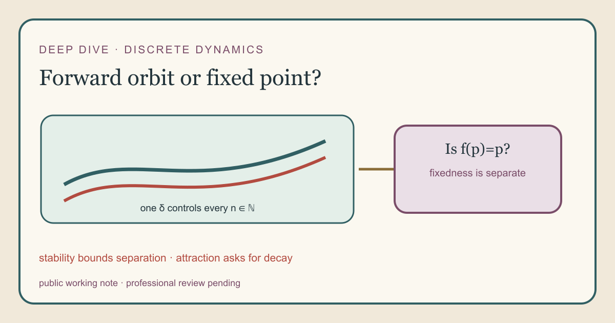
A calculation before the definition
Take \(f(x)=x+2\). Compare starts \(p=4\) and \(x=4.1\):
\[ \begin{array}{c|cc|c} n & f^n(p) & f^n(x) & |f^n(x)-f^n(p)|\\ \hline 0 & 4 & 4.1 & 0.1\\ 1 & 6 & 6.1 & 0.1\\ 2 & 8 & 8.1 & 0.1\\ 3 & 10 & 10.1 & 0.1 \end{array} \]Adding the same constant to both states preserves their difference. The gap is therefore \(0.1\) at every forward time, not only at the four displayed times. The table checks four cases; the algebraic identity establishes the all-time claim for this translation family.
The point \(p=4\) is not fixed because \(f(4)=6\). Stability here belongs to the moving orbit \(4,6,8,10,\ldots\), not to a stationary equilibrium.
Read the quantifiers in order
For a metric-space self-map, forward stability at \(p\) says
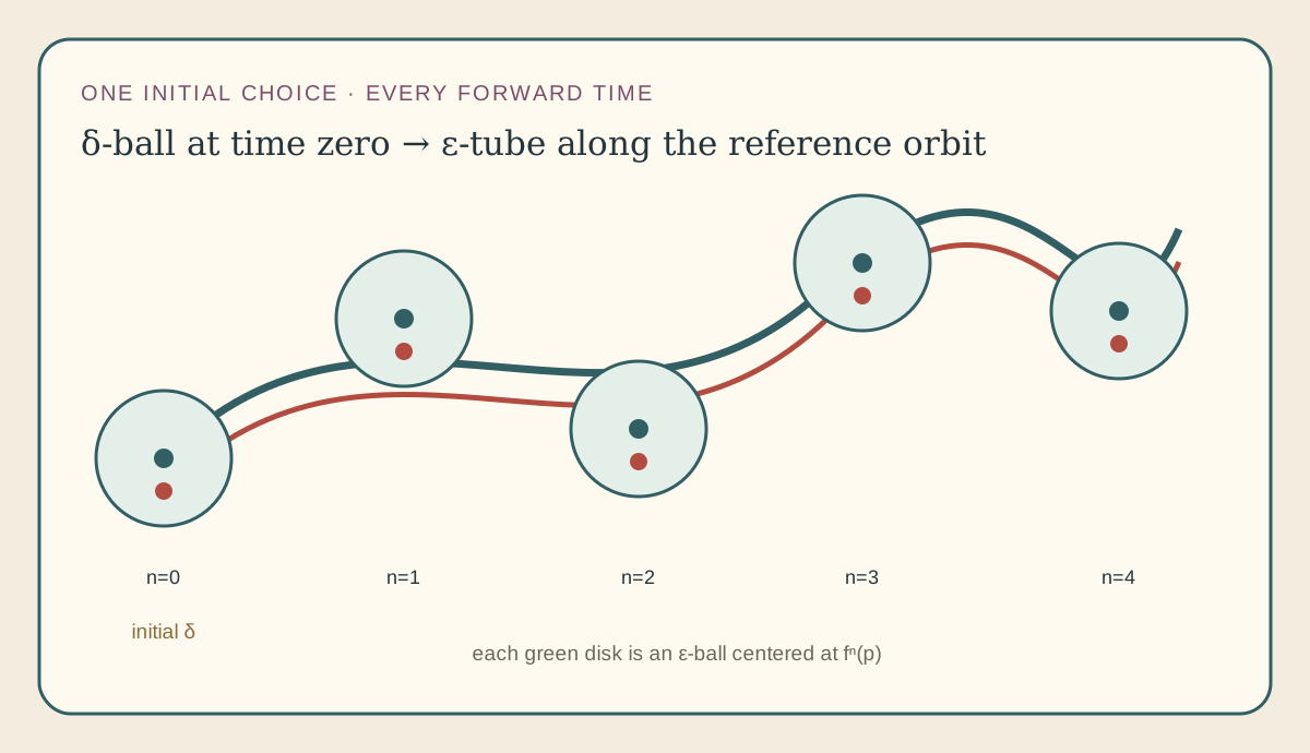
\[ \forall \varepsilon\gt0,\quad \exists\delta\gt0,\quad \forall x,\quad d(x,p)\lt\delta\Longrightarrow \forall n\in\mathbb N,\quad d(f^n(x),f^n(p))\lt\varepsilon. \]The observer chooses the allowed error \(\varepsilon\). Stability responds with one initial radius \(\delta\). Every start inside that ball must work, and the same radius must control every forward time.
That final clause is stronger than checking a fixed list of times. It is also stronger than continuity of each iterate separately, because those continuity arguments may choose radii that shrink as \(n\) grows.
Time zero is included. Since \(f^0\) is the identity, the estimate at \(n=0\) requires the start to lie in the epsilon ball. Choosing \(\delta\le\varepsilon\) is compatible with that boundary.
Why equicontinuity fits
A family \(F_n:X\to X\) is equicontinuous at \(p\) when one initial neighborhood controls every family member. Setting \(F_n=f^n\) produces the forward-stability quantifiers.
Mathlib states equicontinuity for a topological source and uniform-space target. A uniform space specifies uniformly close pairs through entourages. Here the source and target are both \(X\), so one uniform-space structure also supplies its induced topology.
def IsForwardStableAt [UniformSpace X]\n (f : X → X) (p : X) : Prop :=\n EquicontinuousAt (fun n : ℕ ↦ f^[n]) pfun n : ℕ ↦ … builds a natural-number-indexed family.
f^[n] is function iteration, not numerical exponentiation.
p is the point where the entire family is equicontinuous.The theorem isForwardStableAt_iff exposes the entourage form.
isForwardStableAt_iff_dist turns the same predicate into the
epsilon-delta form for pseudo-metric spaces.
Add fixedness only when needed
A fixed point satisfies \(f(p)=p\), so \(f^n(p)=p\) for every \(n\). At a fixed point, the moving-center estimate becomes
\[ d(f^n(x),p)\lt\varepsilon. \]The project defines IsLyapunovStableFixedPoint as fixedness
together with forward stability. The theorem
isLyapunovStableFixedPoint_iff_dist checks the metric form in both
directions.
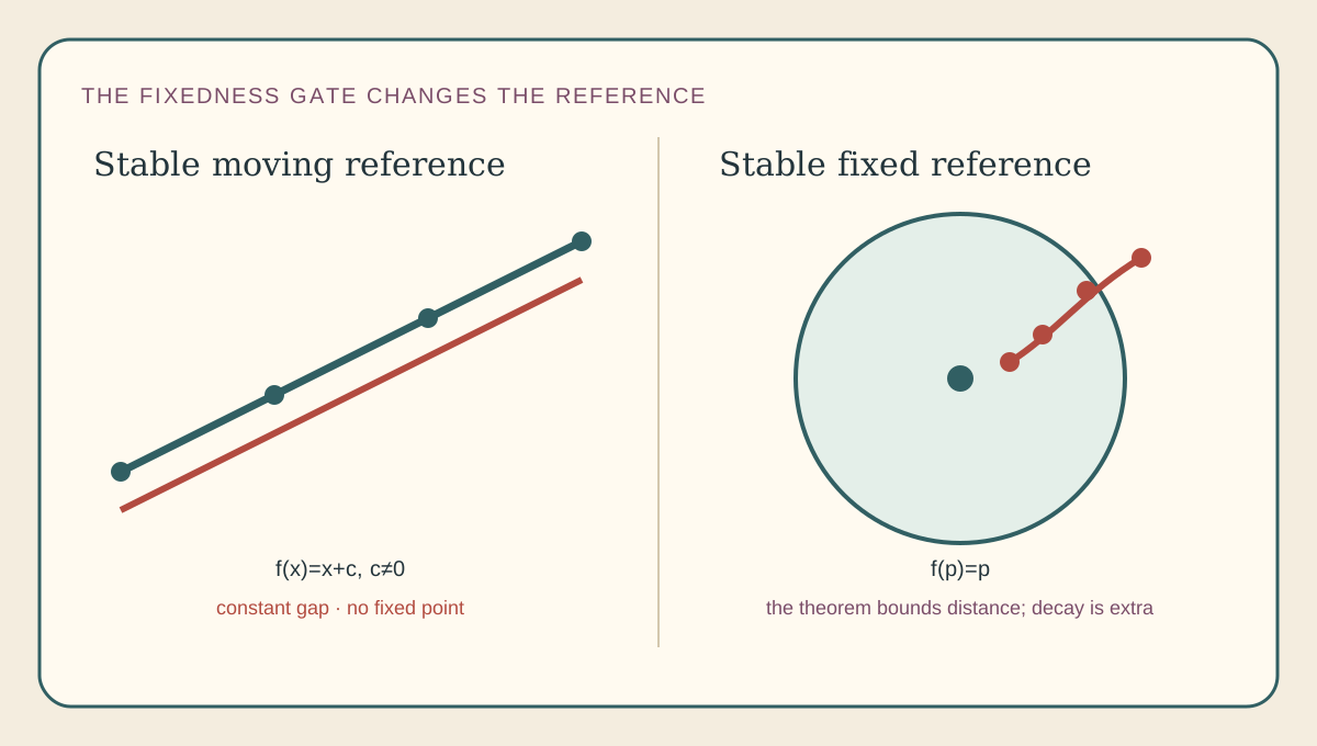
Fixedness cannot be inferred from forward stability.
forwardStableAt_add_const_not_fixed assumes a nonzero translation
amount and returns forward stability together with failure of fixedness.
Nonexpansion supplies the estimate
Suppose \(f\) is nonexpansive:
\[ d(f(x),f(y))\le d(x,y). \]Iteration gives \(d(f^n(x),f^n(y))\le d(x,y)\). Given
\(\varepsilon\gt0\), choose \(\delta=\varepsilon\). This proves
isForwardStableAt_of_lipschitzWith_one from
LipschitzWith 1 f.
The fixed-point wrapper
isLyapunovStableFixedPoint_of_lipschitzWith_one does not discover
a fixed point; it takes fixedness separately. The identity and translation
examples use the nonexpansive result. The constant-map theorem supplies a
fixed point at its constant value.
A standalone Lean worksheet
The bundled translation-gap.lean is a standalone tutorial. It
imports only Std, defines an integer translation orbit, proves its
closed formula by induction, and proves preservation of the gap.
import Std

def translationOrbit (c x : Int) : Nat → Int
  | 0 => x
  | n + 1 => translationOrbit c x n + c

theorem translationOrbit_gap (c x y : Int) :
    ∀ n, translationOrbit c y n - translationOrbit c x n = y - x := by
  intro n
  induction n with
  | zero => rfl
  | succ n ih =>
      simp only [translationOrbit]
      omega
Run it on macOS or Linux with Lean and Std installed:
lean translation-gap.lean
The theorem is general over integer \(c,x,y\) and every natural-number time. The worksheet does not formalize epsilon-delta topology; the Mathlib-backed project module does that.
For the full project check, install the repository’s pinned dependencies:
cd formalization
lake env lean -DwarningAsError=true \
  NonlinearDynamics/Deterministic/Discrete/Stability.lean
lake env selects the pinned environment. The full check may
require substantial disk space and build time on either macOS or Linux.
Stability is not attraction
Stability bounds separation. Attraction requires distance to a target to tend to zero, or a comparable long-time neighborhood property. Translation is forward stable while retaining a constant gap, so it is not an attraction example.
The module also makes no invariant-set claim. Replacing one reference point by a set requires distance-to-set or neighborhood-of-set definitions plus an invariance condition. That belongs to the attraction layer.
This is not structural or stochastic stability either. Those notions vary an update rule or probabilistic object. Here \(f\) is fixed; only the initial state varies. There is also no two-sided-time theorem, exponential estimate, Lyapunov-function criterion, or stable-manifold conclusion.
For a compact review, continue to Forward Stability. For the declaration map and axiom audit, read Forward-Orbit Stability for Discrete Systems in Lean. Then see Lyapunov Functions and the Direct Method in Discrete Time for the checked scalar-certificate layer.
References
- Ethan Akin, “On Chain Continuity,” DCDS 2(1), 111–120 (1996), doi:10.3934/dcds.1996.2.111.
- Saber Elaydi and H. R. Farran, “On Variation of Equicontinuity in Dynamical Systems,” Bull. Aust. Math. Soc. 42(3), 391–397 (1990), doi:10.1017/S0004972700028550.
- J. P. LaSalle, The Stability of Dynamical Systems, Chapter 1, SIAM (1976), doi:10.1137/1.9781611970432.ch1.
- Mathlib, Equicontinuity source, pinned revision
81a5d257.