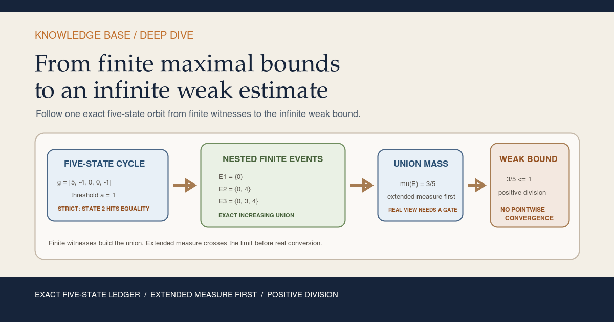
Start with five states you can calculate by hand
Let
\[ \Omega=\{0,1,2,3,4\}, \qquad T(i)=i+1\pmod 5, \qquad \mu(\{i\})=\frac15. \]The map moves around one five-state cycle, and every state has equal mass. Choose the observable
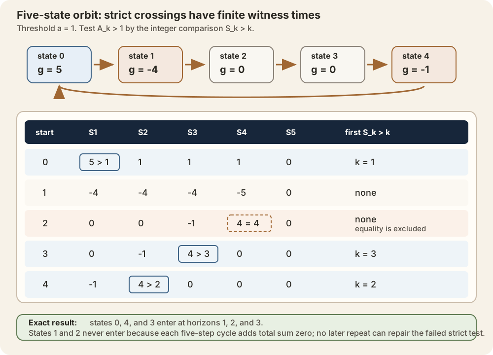
\[ \bigl(g(0),g(1),g(2),g(3),g(4)\bigr) {} = (5,-4,0,0,-1) \]and the strict threshold \(a=1\). Starting at state \(\omega\), write
\[ S_k(\omega) {} = \sum_{j=0}^{k-1}g\bigl(T^j\omega\bigr), \qquad A_k(\omega)=\frac{S_k(\omega)}{k}. \]Because \(k\gt0\),
\[ A_k(\omega)\gt1 \quad\Longleftrightarrow\quad S_k(\omega)\gt k. \]This integer comparison lets us enumerate the event without decimal rounding. The first five partial sums from each starting state are:
| Start \(\omega\) | \(S_1\) | \(S_2\) | \(S_3\) | \(S_4\) | \(S_5\) | First strict witness |
|---|---|---|---|---|---|---|
| \(0\) | \(5\) | \(1\) | \(1\) | \(1\) | \(0\) | \(k=1\), since \(5\gt1\) |
| \(1\) | \(-4\) | \(-4\) | \(-4\) | \(-5\) | \(0\) | none |
| \(2\) | \(0\) | \(0\) | \(-1\) | \(4\) | \(0\) | none; \(S_4=4\) is equality |
| \(3\) | \(0\) | \(-1\) | \(4\) | \(0\) | \(0\) | \(k=3\), since \(4\gt3\) |
| \(4\) | \(-1\) | \(4\) | \(0\) | \(0\) | \(0\) | \(k=2\), since \(4\gt2\) |
The equality in the state-two row is the threshold boundary. The event uses \(A_k\gt1\), so \(A_4(2)=1\) does not count.
Why can we stop the search for states one and two? One full cycle has sum
\[ 5-4+0+0-1=0. \]Writing \(k=5q+r\), each complete cycle contributes zero, so the \(k\)-step sum is just the first \(r\)-step remainder sum. For states one and two, every such remainder satisfies \(S_r\le r\). Since \(r\le5q+r=k\), neither state can cross at a later time. This proves the infinite event exactly; it is not merely a search through the first five steps.
The finite events form an increasing family
Let
\[ E_N {} = \{\omega:\exists k,\ 1\le k\le N \text{ and }1\lt A_k(\omega)\}. \]The ledger gives every finite event:
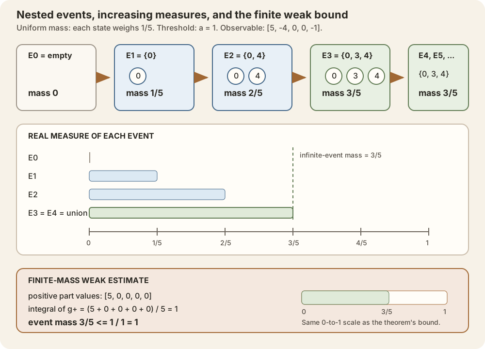
\[ \begin{aligned} E_0&=\varnothing,\\ E_1&=\{0\},\\ E_2&=\{0,4\},\\ E_3&=\{0,3,4\},\\ E_N&=\{0,3,4\}\qquad(N\ge3). \end{aligned} \]The sets are nested because a witness available by horizon \(N\) is still available at every later horizon. Their measures are
\[ 0,\quad\frac15,\quad\frac25,\quad\frac35,\quad\frac35,\ldots \]These are first the native extended-measure values in
\(\mathbb R_{\ge0\infty}\). All are finite in this example, so applying
Measure.real returns the same numerical sequence in
\(\mathbb R\).
Their exact union is
\[ E_1\cup E_2\cup E_3\cup\cdots {} = \{0,3,4\}. \]This is the infinite-horizon event: a point belongs when some finite positive time supplies a strict crossing. The word infinite describes the unbounded search range, not an infinitely long witness.
Check the weak estimate numerically
The positive part of the observable is
\[ \bigl(g^+(0),g^+(1),g^+(2),g^+(3),g^+(4)\bigr) {} = (5,0,0,0,0). \]Therefore
\[ \int_\Omega g^+\,d\mu {} = \frac{5+0+0+0+0}{5} {} = 1. \]The infinite event has real measure \(3/5\). At \(a=1\), the multiplication bound and the divided weak estimate both read
\[ 1\cdot\frac35\le1, \qquad \frac35\le\frac11. \]Every number in this calculation is exact. The example is a probability space for convenience, but the Lean theorem needs only finite total mass, not normalization to one.
What the example has already shown
The finite calculation contains the entire proof architecture:
- every infinite-event member carries one finite positive witness;
- finite events increase with the search horizon;
- their union is the infinite event;
- their measures approach the union measure;
- a horizon-independent finite bound survives the limit; and
- a positive threshold permits division.
The general theorem must now reproduce those moves without assuming a finite state space or eventual stabilization. Its native measure values may include infinity, which creates one important type boundary.
A finite maximal estimate answers a bounded search question: up to horizon \(N\), how large can the set be on which some orbit average exceeds a fixed threshold? Uniformity in \(N\) is essential, but it does not by itself identify the set searched over all positive times.
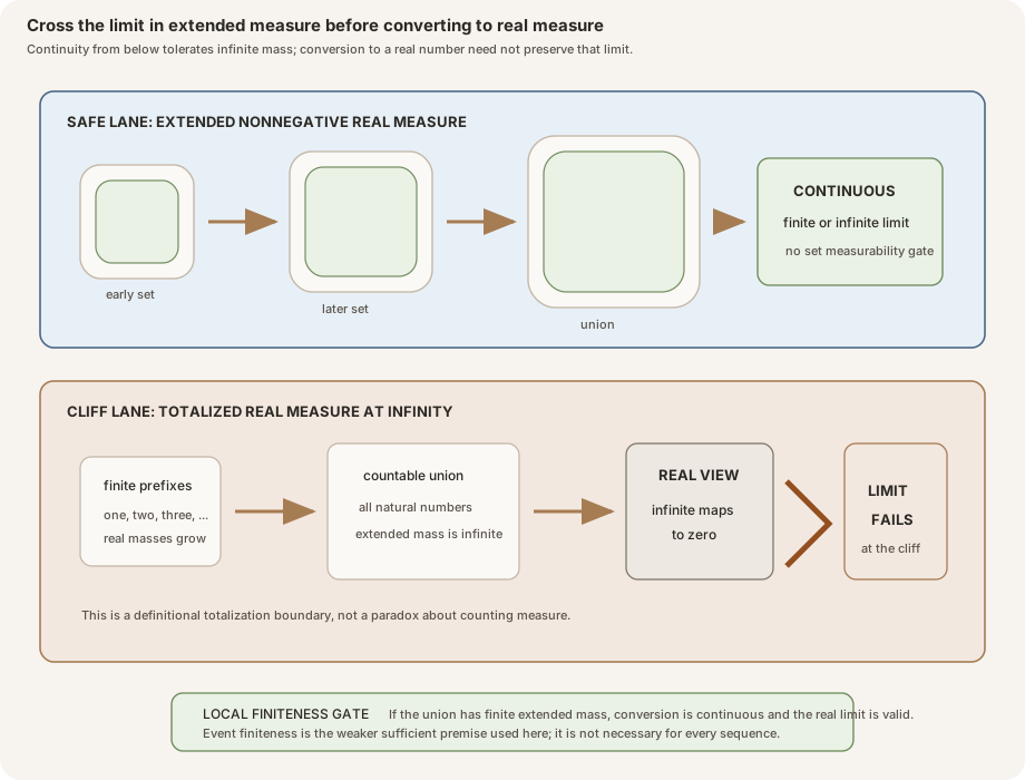
The analytic trap appears when passing to the union. Measures in Lean take
values in the extended nonnegative reals, where infinity is legitimate and
continuity from below is safe. The convenient real-valued view
Measure.real sends infinite mass to zero. Extended convergence
therefore does not automatically survive that projection. RMT-24 exposes
unconditional convergence in extended measure, then a reusable real-valued
corollary under local finiteness. Paired infinite-mass probes show that the
projection can either preserve or destroy a particular limit, so local
finiteness is presented as sufficient rather than necessary.
The compact recurring-concept page is infinite-horizon Birkhoff-average exceedance event . The declaration-complete implementation narrative is Infinite-Horizon Birkhoff-Average Exceedance Bounds in Lean. The finite theorem that supplies the uniform input is Finite Maximal Ergodic Inequalities: From Orbit Maxima to Threshold Events.
Choose a route up
| Route | Begin | Destination |
|---|---|---|
| Worked-example route | Start with five states | Recompute every event and exact mass |
| Event route | Define existence directly | Understand strictness and positive time |
| Set route | Prove the exact increasing union | Build the finite-to-infinite bridge |
| Regularity route | Keep two measurability routes separate | Track ordinary versus null measurability |
| Measure route | Cross the limit in extended measure | Use continuity from below without finiteness |
| Cliff route | Why the checked real-measure theorem uses a local finiteness gate | Diagnose totalization at infinity without overstating necessity |
| Inequality route | Pass the all-threshold bound to the union | Preserve the uniform finite estimate |
| Division route | Divide only at a positive threshold | Obtain the weak maximal estimate |
| History route | Three scopes that must not be merged | Separate source lineage from the checked proof |
| Lean route | The ten-declaration interface | Audit every public name |
| Boundary route | Ten probes protect the theorem | Test degenerate and paired infinite-mass cases |
| Practice route | Solved exercises | Rebuild the argument independently |
| Summit route | What the weak estimate still does not prove | Locate the next pointwise milestone |
Learning objectives
By the summit, a reader should be able to:
- state the positive-time infinite average-exceedance event;
- explain why the threshold comparison is strict;
- explain why time zero is excluded;
- distinguish an existential event from an infinite real maximum;
- recover a finite horizon from an infinite-event witness;
- prove the finite-to-infinite inclusion;
- prove the exact union equality;
- prove that finite events increase with their horizon;
- identify the horizon-zero boundary;
- derive the zero-observable event for both threshold signs;
- derive ordinary measurability from measurable dynamics and observable;
- derive null measurability from preservation and integrability;
- explain why the two regularity routes are not interchangeable labels;
- state continuity from below in extended measure;
- explain why that theorem needs no set measurability here;
- explain why it needs no finite-mass premise;
- define Mathlib’s real-valued measure view;
- prove that this view sends infinite mass to zero;
- construct the counting-measure countermodel to real continuity;
- distinguish local event finiteness from finite total measure;
- pass a uniform finite inequality through a convergent sequence;
- explain why multiplication by a negative threshold need not be monotone;
- explain why monotonicity is unnecessary in the checked limit proof;
- state the multiplication bound for every real threshold;
- identify why negative and zero thresholds may make it uninformative;
- locate the exact premise needed for order-preserving division;
- state the positive-threshold infinite weak estimate;
- audit the full theorem assumption ladder;
- explain why probability normalization is absent;
- explain why ergodicity and invertibility are absent;
- compare Yosida-Kakutani’s historical theorem with this module;
- compare Keane-Petersen’s probability-space development with this module;
- identify the exact scope of the RMT-24 proof rather than attributing it line by line to either source;
- map all ten public declarations to their mathematical roles;
- interpret all ten compiled boundary probes; and
- list the pointwise, strong-type, subadditive, and Lyapunov conclusions that remain unproved.
Common setup and notation
Let:
- \(\Omega\) be a type;
- \(\mu\) be a measure on \(\Omega\) when a measure is needed;
- \(T:\Omega\to\Omega\) be a discrete-time transformation;
- \(T^j\) denote the \(j\)-fold iterate of \(T\);
- \(g:\Omega\to\mathbb R\) be a real observable;
- \(\omega\in\Omega\) be a starting point;
- \(k,N\in\mathbb N\) be a witness time and a finite horizon; and
- \(a\in\mathbb R\) be a fixed threshold.
The finite Birkhoff sum and positive-time average are
\[ S_k g(\omega) {} = \sum_{0\le j\lt k}g\bigl(T^j\omega\bigr), \qquad A_k g(\omega) {} = \frac{S_k g(\omega)}{k} \quad(k\ge1). \]These formulas use Mathlib’s checked finite Birkhoff-sum and average API (Mathlib Birkhoff definitions and boundary lemmas).
The finite average-exceedance event is
\[ E_{N,a}(g) {} = \left\{\omega: \exists k,\quad 1\le k\le N \ \text{and}\ a\lt A_k g(\omega) \right\}. \]RMT-23 proves, on a finite measure space with measure-preserving \(T\) and integrable \(g\), that
\[ a\,\mu_{\mathbb R}\bigl(E_{N,a}(g)\bigr) \le \int_\Omega g^+\,d\mu \qquad\text{for every }N\text{ and every }a\in\mathbb R, \]where \(g^+(\omega)=\max\{g(\omega),0\}\) and \(\mu_{\mathbb R}(S)=\operatorname{toReal}(\mu(S))\). The right side is independent of \(N\). RMT-24 begins exactly from that horizon-uniform fact.
Define existence directly
The infinite event is
\[ E_a(g) {} = \left\{\omega: \exists k\in\mathbb N,\quad 1\le k \ \text{and}\ a\lt A_k g(\omega) \right\}. \]In Lean: name exactly one finite witness
ω ∈ birkhoffAverageExceedanceSet T g a ↔ ∃ k, 1 ≤ k ∧ a < birkhoffAverage ℝ T g k ωω ∈ ...is ordinary set membership.∃ kasks for one natural-number witness; it does not construct an infinite supremum.1 ≤ kremoves the totalized zero-time average.a < ...encodes a strict crossing, so equality stays outside.birkhoffAverage ℝ T g k ωis the real \(k\)-step average of \(g\) along the orbit of \(\omega\).
The exact source definition is:
def birkhoffAverageExceedanceSet
    (T : Ω → Ω) (g : Ω → ℝ) (a : ℝ) : Set Ω :=
  {ω | ∃ k, 1 ≤ k ∧ a < birkhoffAverage ℝ T g k ω}
The companion
mem_birkhoffAverageExceedanceSet_iff exposes the displayed
membership statement by reflexivity.
This formulation has three advantages.
First, it says precisely what the weak estimate needs: existence of one threshold crossing. It makes no demand that the averages be bounded above, so there is no need to choose between a real supremum, an extended-real supremum, or an arbitrary totalization convention.
Second, positivity of the time is visible. The zero-time Birkhoff average is totalized in Lean, but it is not an observed average. A witness must satisfy \(1\le k\).
Third, the comparison is strict. Equality \(A_k g(\omega)=a\) is not a crossing. This sidedness matches the strict finite maximal event from RMT-23. Changing it would change the event on threshold atoms and would no longer be the same theorem interface.
The membership theorem
mem_birkhoffAverageExceedanceSet_iff is definitionally exact. It
does not need a measurable space. That apparently small fact matters: the
set-theoretic bridge can be proved before any analytic assumptions are chosen.
A worked sign calibration
Take \(g(\omega)=0\) for every \(\omega\). Every positive-time average equals zero. Therefore
\[ E_a(0) {} = \begin{cases} \varnothing, & 0\le a,\\ \Omega, & a\lt0. \end{cases} \]At \(a=0\), strictness chooses the empty branch. At \(a=-1\), time one is a witness for every point. These two compiled examples prevent prose from quietly replacing strict exceedance by nonstrict exceedance.
Prove the exact increasing union
The central set identity is
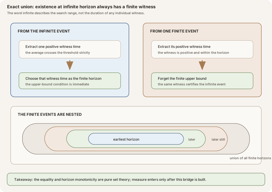
\[ E_a(g)=\bigcup_{N\in\mathbb N}E_{N,a}(g). \]Start with \(\omega\in E_a(g)\). By membership, there is a positive natural time \(k\) with \(a\lt A_k g(\omega)\). Choose the finite horizon \(N=k\). Then \(1\le k\le N\), so \(\omega\in E_{k,a}(g)\), and hence \(\omega\) lies in the union.
For the reverse inclusion, suppose \(\omega\in E_{N,a}(g)\) for some \(N\). There is a time \(k\) satisfying \(1\le k\le N\) and \(a\lt A_k g(\omega)\). Forgetting \(k\le N\) leaves exactly the witness required for \(\omega\in E_a(g)\).
In Lean: turn the unbounded search into an exact union
birkhoffAverageExceedanceSet_eq_iUnion_finite (T := T) (g := g) a⋃ N : ℕ, ...is a countable union indexed by finite horizons.- The forward proof extracts
k, then chooses the same value as the union index and finite horizon. - The reverse proof keeps the witness
kand forgets only the conditionk ≤ N. - The equality is literal
Setequality. There is noAlmostEverywherequalifier and no measure in the statement.
The theorem statement is:
theorem birkhoffAverageExceedanceSet_eq_iUnion_finite (a : ℝ) :
    birkhoffAverageExceedanceSet T g a =
      ⋃ N : ℕ, finiteBirkhoffAverageExceedanceSet T g N a
There is no limiting argument in this equality.
The theorem is exact as sets, not only modulo null sets. It requires neither a
measurable space nor a measure. The companion theorem
finiteBirkhoffAverageExceedanceSet_subset packages the
finite-to-infinite inclusion for later reuse.
The finite events are increasing because increasing \(N\) only relaxes the upper witness bound. RMT-23 already proves
\[ M\le N \quad\Longrightarrow\quad E_{M,a}(g)\subseteq E_{N,a}(g). \]This is monotonicity of events by search horizon. It says nothing about whether the average sequence \(A_k g(\omega)\) rises or falls along any one orbit.
Why horizon zero is harmless
At \(N=0\), the finite event is empty because there is no \(k\) with
\(1\le k\le0\). The union nevertheless starts at zero. An empty first term is
convenient: the index type remains all natural numbers, Mathlib’s
atTop continuity theorem applies directly, and no artificial
successor reindexing is needed.
Keep two measurability routes separate
The event is useful in settings with different available regularity. RMT-24 therefore proves ordinary measurability and null measurability by separate routes.
Route one: ordinary measurability
Assume \(T\) and \(g\) are measurable. Every iterate \(T^j\) is measurable, every finite Birkhoff sum and average is measurable, and every finite strict superlevel event \(E_{N,a}(g)\) is measurable. The exact union is countable, so
\[ \operatorname{MeasurableSet}\bigl(E_a(g)\bigr). \]The public theorem is
measurableSet_birkhoffAverageExceedanceSet. It consumes ordinary
measurability and returns an ordinary measurable set. It needs no measure,
integrability, preservation, finite mass, probability, or ergodicity.
Route two: null measurability from integrability
Now suppose \(T\) preserves \(\mu\) and \(g\) is integrable with respect to \(\mu\). Integrability supplies almost-everywhere strong measurability of \(g\), not necessarily ordinary measurability of the chosen pointwise representative. Preservation transports integrability along each orbit iterate, so every positive-time Birkhoff average is integrable.
RMT-24 rewrites the event as a union indexed by the subtype of positive natural times:
\[ E_a(g) {} = \bigcup_{k\ge1} \{\omega:a\lt A_k g(\omega)\}. \]Each average is almost-everywhere measurable, the constant threshold is measurable, and each strict comparison set is null measurable. A countable union of null-measurable sets is null measurable. Thus
\[ \operatorname{NullMeasurableSet}_\mu\bigl(E_a(g)\bigr). \]This theorem is named
nullMeasurableSet_birkhoffAverageExceedanceSet_of_integrable. It
requires no finite total mass. Counting measure on the natural numbers is an
explicit compiled probe of that claim.
Do not relabel one route as the other
An ordinarily measurable set is null measurable, but the reverse statement
need not hold for the exact representative. Null measurability says that the
set agrees with some measurable set outside a null set. It is enough for its
measure and for many almost-everywhere arguments, but it is not an ordinary
MeasurableSet certificate.
The two theorem statements also expose different sources of regularity:
| Goal | Premises | Premises not used |
|---|---|---|
| Ordinary measurable event | Measurable \(T\), measurable \(g\) | Any measure, integrability, preservation, finite mass |
| Null-measurable event | Measure-preserving \(T\), integrable \(g\) | Ordinary measurability of the chosen \(g\), finite mass, probability, ergodicity |
Measure preservation already includes measurability of \(T\). The second route does not treat preservation as an ergodicity or invertibility hypothesis.
Cross the limit in extended measure
Let
\[ m_N=\mu\bigl(E_{N,a}(g)\bigr) \quad\text{and}\quad m=\mu\bigl(E_a(g)\bigr), \]where these values lie in the extended nonnegative reals \(\mathbb R_{\ge0\infty}\). Since the events increase with \(N\) and their union is \(E_a(g)\), continuity from below gives
\[ m_N\longrightarrow m. \]In Lean: take the limit before leaving extended measure
tendsto_measure_finiteBirkhoffAverageExceedanceSet (T := T) (g := g) (μ := μ) aTendstois Lean’s filter-level statement of convergence.fun N ↦ μ (...)is the sequence of native measure values inENNReal.atTopmeans that the natural horizon tends upward without bound.nhds (μ (...))names the neighborhoods of the union’s measure.- No
IsFiniteMeasure, ordinary measurability, preservation, or integrability hypothesis appears in the theorem.
The checked statement is:
theorem tendsto_measure_finiteBirkhoffAverageExceedanceSet (a : ℝ) :
    Tendsto
      (fun N ↦ μ (finiteBirkhoffAverageExceedanceSet T g N a))
      atTop (nhds (μ (birkhoffAverageExceedanceSet T g a)))
Its assumptions are intentionally minimal. It needs the ambient measurable
space because a Measure is typed over one, but it assumes no
measurability of \(T\), \(g\), or the events. It assumes no integrability,
preservation, finite mass, probability, or ergodicity.
That boundary is supported by Mathlib’s exact theorem
tendsto_measure_iUnion_atTop
(continuity from below), whose documentation explicitly
allows increasing sets that are not necessarily measurable. The limit may be
infinite. Extended measure is the native codomain for which continuity from
below remains valid at infinite mass.
Why the checked real-measure theorem uses a local finiteness gate
Mathlib defines
\[ \mu_{\mathbb R}(S) {} = \operatorname{toReal}\bigl(\mu(S)\bigr). \]This is the exact Measure.real definition.
For finite extended values, toReal is the expected conversion.
At infinity, it returns zero:
Therefore the map is not continuous at infinity. RMT-24 states a clean, reusable sufficient corollary under
\[ \mu\bigl(E_a(g)\bigr)\ne\infty. \]Under that local hypothesis, ENNReal.tendsto_toReal
(continuity of toReal at a finite target) composes with
extended-measure continuity and yields
In Lean: convert only at a finite target
tendsto_measureReal_finiteBirkhoffAverageExceedanceSet (T := T) (g := g) (μ := μ) a hfinitehfinitehas the local typeμ (birkhoffAverageExceedanceSet T g a) ≠ ∞.μ.real Sunfolds to(μ S).toReal.ENNReal.tendsto_toReal hfinitesupplies continuity of that conversion at this finite target..compcomposes it with the preceding extended-measure convergence.- The premise concerns the one union event, not the total mass of \(\Omega\).
The finite-target theorem is sufficient for a reusable interface. It does not claim that every infinite-target sequence fails after conversion.
A finite measure space makes the premise automatic, while local event finiteness is the weaker of those two sufficient interfaces. Neither is claimed to be necessary for every particular increasing family.
Infinite mass: one failure and one near miss
Failure: finite prefixes approach an infinite union
Let \(\mu\) be counting measure on \(\mathbb N\), and define
\[ F_N=\{n\in\mathbb N:n\lt N\}. \]The sets increase and \(\bigcup_NF_N=\mathbb N\). Each finite set has
\[ \mu_{\mathbb R}(F_N)=N. \]The union has infinite extended measure:
\[ \mu(\mathbb N)=\infty. \]Its totalized real measure is therefore
\[ \mu_{\mathbb R}(\mathbb N) {} = \operatorname{toReal}(\infty) {} = 0. \]The sequence \(N\) does not converge to zero. Thus real-valued continuity from below can fail when the limiting extended mass is infinite. RMT-24 includes this countermodel as compiled Lean code, so no unconditional conversion theorem is available.
Near miss: the totalized real sequence still converges
Failure is not forced by infinite mass. With counting measure, identity
dynamics, constant observable two, and threshold one, every finite event from
horizon one onward and the infinite event are univ. Their
totalized real measures are all zero, hence the real sequence converges even
though the extended union mass is infinite. A second compiled probe checks this
event-family example. Together the probes show that local finiteness is a clean
sufficient theorem premise, not an if-and-only-if characterization.
Why the totalization is not a contradiction
The equality \(\operatorname{toReal}(\infty)=0\) is a design choice for a total function from an extended type to \(\mathbb R\). It does not claim that an infinite set has ordinary real mass zero. The extended value remains \(\infty\); information is lost only when one insists on a total real-valued projection. This proof therefore establishes a finite target before it uses that projection as a faithful numerical measure; an infinite target requires separate information.
Pass the all-threshold bound to the union
Assume from now on:
- \(\mu\) has finite total mass;
- \(T\) preserves \(\mu\); and
- \(g\) is integrable with respect to \(\mu\).
Write
\[ I^+(g)=\int_\Omega g^+\,d\mu, \qquad g^+(\omega)=\max\{g(\omega),0\}. \]RMT-23 provides, for every natural horizon \(N\) and every real threshold \(a\),
\[ a\,\mu_{\mathbb R}\bigl(E_{N,a}(g)\bigr) \le I^+(g). \]Finite total mass makes \(\mu(E_a(g))\ne\infty\), so the real measures of the finite events converge to the real measure of the union. Multiplying that convergent sequence by the fixed real constant \(a\) gives
\[ a\,\mu_{\mathbb R}\bigl(E_{N,a}(g)\bigr) \longrightarrow a\,\mu_{\mathbb R}\bigl(E_a(g)\bigr). \]Every term is at most \(I^+(g)\), and a limit of values bounded above by the same constant retains that upper bound. Hence
\[ a\,\mu_{\mathbb R}\bigl(E_a(g)\bigr) \le I^+(g). \]In Lean: pass the common finite bound through the limit
birkhoffAverageExceedanceSet_posPart_bound hT hg a[IsFiniteMeasure μ]supplies finite total mass.hT : MeasurePreserving T μ μandhg : Integrable g μare the analytic inputs inherited by every finite estimate.- The argument
ais any real number; positivity is not yet required. max (g ω) 0is the pointwise positive part.- The proof multiplies a convergent real-measure sequence by the fixed
constant and uses
le_of_tendsto'to preserve the common upper bound.
The theorem does not assert that the products are monotone.
Why no sign premise is needed here
The theorem accepts every \(a\in\mathbb R\). The proof does not argue that the products \(a\,\mu_{\mathbb R}(E_{N,a})\) increase with \(N\). That would be false as a general monotonicity claim when \(a\lt0\), because multiplying an increasing nonnegative sequence by a negative constant reverses order.
Instead, the proof uses continuity of multiplication by the fixed constant
\(a\), then transfers the common upper bound through the limit with
le_of_tendsto’. This argument is valid for every real \(a\).
At \(a\lt0\), the left side is nonpositive and the right side is nonnegative, so the inequality may be automatic and uninformative. At \(a=0\), it reduces to \(0\le I^+(g)\). Validity for all thresholds and usefulness for all thresholds are different claims.
Why finite total mass appears
Finite total mass performs two jobs in this theorem.
First, the RMT-23 threshold argument applies the finite Hopf lemma to \(g-a\). Integrability of the constant function \(a\) follows from finite total mass. Without that premise, an arbitrary nonzero constant need not be integrable.
Second, finite total mass discharges the local finiteness premise needed to convert the increasing-event limit to real measure. The sharper real continuity theorem remains separately available when only this particular event is known to have finite mass, but the finite threshold inequality itself still uses the stronger finite-measure context.
Divide only at a positive threshold
Suppose now that \(0\lt a\). Division by \(a\) preserves order, so the multiplication bound becomes
\[ \mu_{\mathbb R}\bigl(E_a(g)\bigr) \le \frac{I^+(g)}{a} {} = \frac{\displaystyle\int_\Omega\max\{g(\omega),0\}\,d\mu(\omega)}{a}. \]In Lean: divide with a proof that the threshold is positive
measureReal_birkhoffAverageExceedanceSet_le hT hg haha : 0 < ais proof data, not a comment or runtime check.le_div_iff₀ hais the order equivalence for division by a positive real.- The result reuses the multiplication theorem and only commutes the two factors to match its conclusion.
- No probability, ergodicity, injectivity, surjectivity, or invertibility assumption is added.
This is the module’s final infinite-horizon weak maximal estimate.
The positivity premise enters exactly in Lean’s
le_div_iff₀ step. At \(a=0\), division would be totalized but
would not recover the event measure from the multiplication inequality. At a
negative threshold, dividing reverses the inequality and does not produce the
claimed upper bound. The theorem therefore states \(0\lt a\), not merely
\(a\ne0\).
The estimate is called weak because it controls the measure of a superlevel event by a first-power tail bound. It is not a strong \(L^p\) norm inequality and does not construct a maximal function as a real-valued member of any \(L^p\) space.
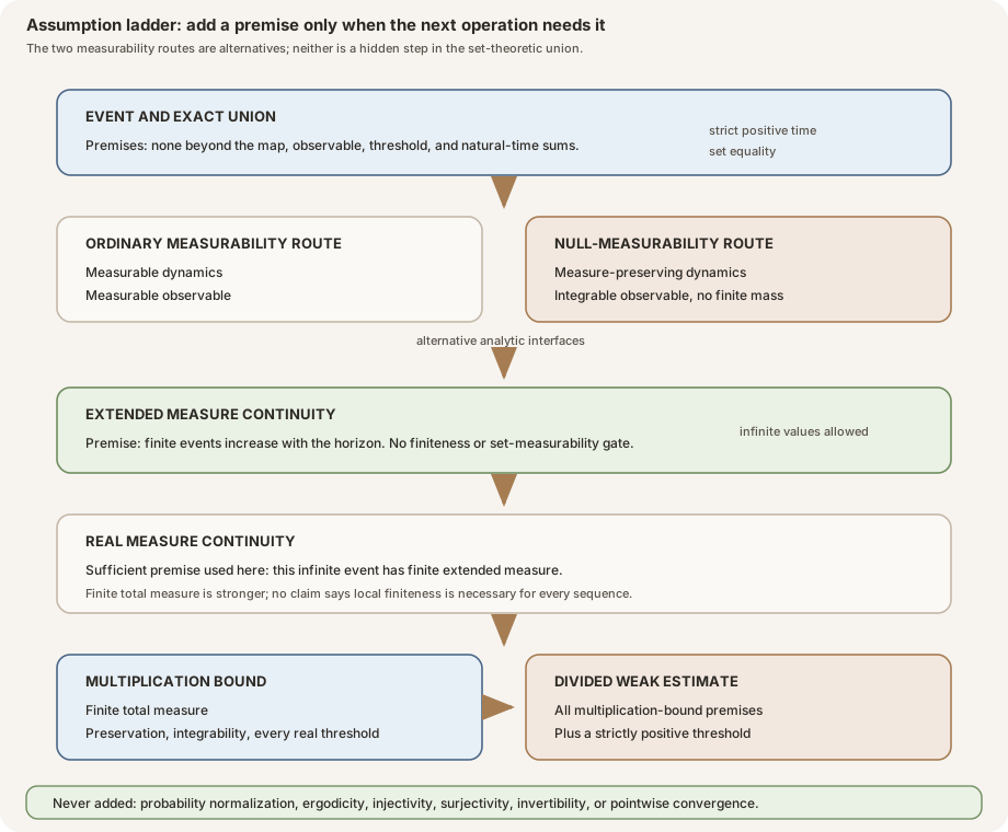
A full assumption ledger
| Layer | Checked result | Required | Explicitly absent |
|---|---|---|---|
| Definition | Positive-time strict exceedance event | Map, observable, real threshold | Measurable space, measure, integrability |
| Membership | Existential witness equivalence | Same raw data | Every analytic premise |
| Exact union | Infinite event equals union of finite events | Natural-time witness arithmetic | Measurability, measure, topology |
| Finite inclusion | Each finite event lies in the infinite event | Same raw data | Every analytic premise |
| Ordinary regularity | Infinite event is measurable | Measurable \(T\), measurable \(g\) | Integrability, preservation, finite mass |
| Null regularity | Infinite event is null measurable | Measure-preserving \(T\), integrable \(g\) | Ordinary measurable \(g\), finite mass, probability |
| Extended limit | Finite event measures tend to the union measure | Increasing finite events | Set measurability, finiteness, dynamics |
| Real limit | Real finite-event measures tend to real union measure | Union event has finite extended mass | Finite total mass as such |
| Multiplication bound | Threshold times event mass bounded by positive-part integral | Finite total measure, preservation, integrability, any real threshold | Positive threshold, probability, ergodicity |
| Weak estimate | Event mass bounded by positive-part integral divided by threshold | All preceding analytic premises and \(0\lt a\) | Invertibility, pointwise convergence, strong type |
The module never requires sigma-finiteness as a separate premise. Finite total measure implies it where needed, but the event-level and extended-continuity theorems do not add it.
Three scopes that must not be merged
Historical sources explain why this route matters, but they do not all state the same theorem or use the same proof.
Yosida and Kakutani: an early infinite-horizon theorem
Yosida and Kakutani’s 1939 article works with a one-to-one measure-preserving point transformation and an integrable real observable, and explicitly does not assume finite total measure in its opening setting. Its Theorem 2 is an infinite-horizon average formulation, and pages 166-167 prove it through finite maximal intervals (Yosida and Kakutani, 1939).
That paper supplies priority and historical scope. RMT-24 does not formalize its one-to-one premise, its maximal-interval selection proof, or its theorem line by line. In particular, the checked Lean module permits noninjective measure-preserving maps and obtains its finite input from RMT-23’s separate maximum-minus-shift argument, whose finite historical lineage runs through Garsia’s proof.
Keane and Petersen: the closest finite-to-infinite precedent
Keane and Petersen’s 2006 note begins on a probability space with an integrable observable and permits a possibly noninvertible measure-preserving transformation. Its maximal theorem allows a threshold \(\lambda\) that is almost everywhere invariant and whose positive part \(\lambda^+\) is integrable. Pages 248-249 form strict finite maximal-average events and pass toward an infinite maximal theorem; the note continues into a nearly simultaneous proof of the pointwise ergodic theorem (Keane and Petersen, 2006).
This is the closest primary precedent for RMT-24’s finite-to-infinite direction. The interfaces are still not identical. RMT-24 separates the raw set equality, ordinary and null measurability, unconditional extended-measure continuity, locally finite real-measure continuity, the all-real-threshold multiplication bound, and positive-threshold division. It uses finite total measure rather than a probability normalization for the final analytic bound. It does not formalize Keane and Petersen’s bounded approximation or pointwise convergence steps.
The checked proof: a project-specific composition
The RMT-24 proof composes four checked ingredients:
- the finite strict average-exceedance events and their horizon monotonicity from RMT-23;
- the exact witness-level union proved in RMT-24;
- Mathlib’s continuity from below in extended measure and continuity of
toRealaway from infinity; and - the RMT-23 horizon-uniform positive-part bound, transferred through the real limit.
This composition is mathematically standard, but the Lean organization and assumption-minimized interface are the project’s own checked proof. It should not be described as a line-by-line formalization of Yosida-Kakutani or Keane-Petersen.
| Source | Ambient setting | Relevant contribution | Not imported as an RMT-24 claim |
|---|---|---|---|
| Yosida-Kakutani 1939 | One-to-one measure-preserving point map and integrable real observable; total mass need not be finite | Early named infinite-horizon theorem and finite maximal-interval route | Injectivity, exact interval proof, or line-by-line theorem identity |
| Keane-Petersen 2006 | Integrable observable and possibly noninvertible measure-preserving map on a probability space; almost everywhere invariant threshold \(\lambda\) with integrable \(\lambda^+\) | Closest finite strict-event to infinite maximal passage | Probability normalization, variable invariant threshold, bounded approximation, or pointwise theorem |
| RMT-23 plus RMT-24 | Measure-preserving map; finite mass only at threshold-bound layer | Maximum-minus-shift finite input, exact union, typed continuity, weak estimate | Any convergence existence or strong maximal theorem |
The ten-declaration interface
The 342-line module has ten documented public declarations, no private helper, and ten anonymous compiled probes.
Pure set layer
birkhoffAverageExceedanceSetdefines the infinite event by a strict crossing at a positive natural time.mem_birkhoffAverageExceedanceSet_iffexposes exactly that witness predicate and omits the ambient measurable-space assumption.birkhoffAverageExceedanceSet_eq_iUnion_finiteproves exact equality with the union of finite events, using the witness time itself as a horizon in one direction.finiteBirkhoffAverageExceedanceSet_subsetpackages the inclusion of each finite event into the infinite event.
Regularity layer
measurableSet_birkhoffAverageExceedanceSetproves ordinary measurability from measurable \(T\) and measurable \(g\).nullMeasurableSet_birkhoffAverageExceedanceSet_of_integrableproves null measurability from preservation and integrability by a countable union over positive times.
Continuity layer
tendsto_measure_finiteBirkhoffAverageExceedanceSetproves unconditional convergence of the extended measures of the increasing finite events to the extended measure of the union.tendsto_measureReal_finiteBirkhoffAverageExceedanceSetcomposes that theorem with real conversion under the local premise that the union’s extended measure is not infinite.
Inequality layer
birkhoffAverageExceedanceSet_posPart_boundpasses the uniform finite bound through the real limit on a finite measure space for every real threshold.measureReal_birkhoffAverageExceedanceSet_ledivides by a strictly positive threshold to obtain the infinite weak estimate.
Private and proof-local inventory
There is no private def, private theorem, private instance, or named
internal declaration in this module. The complete visibility map is therefore:
| Visibility | Names | Reader-facing role |
|---|---|---|
| Public definition | birkhoffAverageExceedanceSet | Names the infinite event |
| Public theorems | The other nine names listed above | Membership, exact union, inclusion, regularity, continuity, and bounds |
| Private declarations | none | There is no hidden callable API |
| Anonymous examples | ten | Compile theorem boundaries without exporting names |
| Proof-local terms | heq, hreal, and local have / let bindings inside probes | Organize individual proofs; they disappear outside their proof bodies |
In particular, heq rewrites the null-measurable event as a
positive-time subtype union, while hreal composes extended
convergence with finite-target real conversion. Neither is a declaration that
downstream code can import.
Five #print axioms commands inspect the null-regularity theorem,
both continuity theorems, and both final inequalities. The module introduces no
custom axiom, proof hole, unsafe declaration, infinite supremum, or hidden
choice of an infinite maximizing time.
Ten probes protect the theorem
The anonymous examples are executable specification tests.
- Witness recovery. Membership in the infinite event yields a concrete finite horizon, chosen as the witness time itself.
- Horizon zero. The finite event at horizon zero is empty.
- Zero observable, nonnegative threshold. Every average is zero, so the strict event is empty.
- Zero observable, negative threshold. Time one witnesses every point, so the event is the whole space.
- Zero measure. The multiplication bound specializes correctly when every set and integral has zero measure.
- Infinite counting measure. The null-measurable event theorem compiles on the natural numbers with counting measure together with an explicit proof that this measure is not finite. Thus finite total mass is absent from that route.
- Positive-threshold division. The public weak estimate can be reused directly under its exact hypotheses.
- Noninjective dynamics. A constant map preserving a Dirac measure, with constant observable two and threshold one, has a positive-mass exceedance event and satisfies the theorem. Thus injectivity and invertibility are not hidden even in a nonvacuous event branch.
- Infinite mass with a successful real limit. Under counting measure, identity dynamics, constant observable two, and threshold one, every event from horizon one onward and the infinite event are the whole space. Their totalized real measures are all zero, so convergence holds despite infinite extended union mass. This proves local finiteness is not necessary for every particular family.
- The real-measure cliff. Increasing finite counting-measure ranges cover all natural numbers, but their real measures do not converge to the totalized real measure of the union. This proves there is no unconditional real-conversion theorem for all increasing families.
Together these probes distinguish theorem premises from habits inherited from probability-space presentations.
Exact claims and nonclaims
| The checked module establishes | It does not establish |
|---|---|
| One strict positive-time threshold crossing defines the infinite event | Existence of a real-valued infinite maximum |
| Exact equality with an increasing union of finite events | Only an almost-everywhere or approximate union |
| Ordinary measurability under ordinary measurable inputs | Ordinary measurability from integrability alone |
| Null measurability from preservation and integrability | Probability normalization or ergodicity |
| Extended-measure continuity without finiteness | An ungated real-measure continuity theorem for every increasing family |
| A sufficient locally finite real-measure continuity theorem | Local finiteness as a necessary condition for every particular family |
| An all-real-threshold multiplication bound under finite total measure | An informative event-size estimate at every nonpositive threshold |
| A positive-threshold weak estimate | A strong \(L^p\) maximal inequality |
| Validity for noninjective measure-preserving maps | Invertibility, surjectivity, or two-sided time |
| One infinite-horizon maximal component | Pointwise or almost-everywhere convergence of Birkhoff averages |
The final row is the most important. A weak bound controls the measure of points with at least one threshold crossing. It does not choose the limiting value of the average sequence and does not show that a limit exists.
Solved exercises
Exercise 1: unpack infinite-event membership
State in words what \(\omega\in E_a(g)\) means. Which quantities are fixed, and which quantity is existentially chosen?
Solution. The transformation \(T\), observable \(g\), threshold \(a\), and starting point \(\omega\) are fixed. Membership means that there exists a natural time \(k\) with \(1\le k\) such that the finite Birkhoff average at that time satisfies \(a\lt A_k g(\omega)\). The witness is the finite positive time \(k\). No limiting time or maximizing time over an infinite set is chosen.
Exercise 2: test the strict boundary
Suppose \(A_k g(\omega)=a\) for one positive time \(k\), and every other positive-time average is at most \(a\). Is \(\omega\in E_a(g)\)?
Solution. No. The event requires a strict inequality \(a\lt A_j g(\omega)\) for at least one positive \(j\). Equality at \(k\) does not qualify, and the hypothesis excludes a strict crossing at every other time. Replacing the event by a nonstrict one would change this answer and would define a different theorem.
Exercise 3: explain the positive-time guard
Why not define the event by \(\exists k,\ a\lt A_k g(\omega)\) and allow \(k=0\)?
Solution. Lean’s field division and Birkhoff average are totalized at zero, but that value is not the average of any observed orbit entries. Its behavior is a convention needed to make the function total. Allowing it as a witness could make membership depend on a boundary convention rather than on positive-time dynamics. The explicit condition \(1\le k\) removes that ambiguity and is also what licenses multiplication by \(k\) in finite threshold translations.
Exercise 4: compute horizon zero
Prove \(E_{0,a}(g)=\varnothing\) without using any property of \(T\), \(g\), or \(a\).
Solution. Membership would require a natural number \(k\) satisfying both \(1\le k\) and \(k\le0\). No natural number has those two properties. Hence there is no witness and the set is empty. The average inequality is never inspected.
Exercise 5: calibrate the zero observable
Let \(g=0\). Determine \(E_a(g)\) when \(a\ge0\) and when \(a\lt0\).
Solution. Every positive-time sum and average equals zero. If \(a\ge0\), the strict inequality \(a\lt0\) is false, so the event is empty. If \(a\lt0\), time one satisfies \(a\lt A_1g(\omega)=0\) for every \(\omega\), so the event is all of \(\Omega\). At \(a=0\), strictness selects the empty case.
Exercise 6: prove the infinite-to-finite inclusion
Given \(\omega\in E_a(g)\), construct an explicit \(N\) such that \(\omega\in E_{N,a}(g)\).
Solution. Extract the witness \(k\) with \(1\le k\) and \(a\lt A_kg(\omega)\). Set \(N=k\). Then \(1\le k\le N\) because the upper inequality is reflexive. The same average inequality proves \(\omega\in E_{k,a}(g)\).
Exercise 7: prove the finite-to-infinite inclusion
Given \(\omega\in E_{N,a}(g)\), prove \(\omega\in E_a(g)\).
Solution. Finite membership supplies \(k\) with \(1\le k\le N\) and \(a\lt A_kg(\omega)\). Infinite membership asks only for \(1\le k\) and the strict average inequality. Discard the upper bound \(k\le N\) and reuse the same witness.
Exercise 8: derive the exact union
Combine Exercises 6 and 7 to prove \(E_a(g)=\bigcup_NE_{N,a}(g)\).
Solution. Exercise 6 shows every point in \(E_a(g)\) belongs to at least one finite event, so the infinite event is contained in the union. Exercise 7 shows every point in every finite event belongs to the infinite event, so the union is contained in the infinite event. Antisymmetry of set inclusion gives equality.
Exercise 9: prove event monotonicity
Suppose \(M\le N\). Show \(E_{M,a}(g)\subseteq E_{N,a}(g)\).
Solution. A point in the smaller-horizon event has a witness \(k\) with \(1\le k\le M\). Transitivity gives \(k\le N\). The strict average inequality is unchanged, so the same witness proves membership at horizon \(N\).
Exercise 10: reject a false monotonicity inference
Does Exercise 9 imply \(A_Mg(\omega)\le A_Ng(\omega)\) for every \(M\le N\)?
Solution. No. Event monotonicity comes from retaining all witness times available at earlier horizons. It does not compare the terminal averages at times \(M\) and \(N\). For example, an orbit can begin with a large positive value and then several negative values, so the averages can decrease even though the set of searched times grows.
Exercise 11: isolate the set-theoretic assumptions
Which assumptions are used in the membership theorem, exact union, and finite inclusion?
Solution. Only the raw functions, natural-time Birkhoff averages, and order relations are used. No measurable space, measure, topology, integrability, measure preservation, probability normalization, ergodicity, or invertibility is required. In Lean, the first three theorems explicitly omit the otherwise ambient measurable-space instance.
Exercise 12: build the ordinary measurable route
Assume \(T\) and \(g\) are measurable. Explain why \(E_a(g)\) is measurable.
Solution. Every iterate of \(T\) is measurable. Finite sums of the measurable functions \(g\circ T^j\) are measurable, and division by the constant natural number at a fixed positive time preserves measurability. Each finite strict average-exceedance event is therefore measurable. The infinite event is their countable union by the exact set identity, and a countable union of measurable sets is measurable.
Exercise 13: build the null-measurable route
Assume \(T\) preserves \(\mu\) and \(g\) is integrable. Why is \(E_a(g)\) null measurable even if the selected representative of \(g\) is not ordinarily measurable?
Solution. Preservation transports integrability through every iterate of \(T\), so every positive-time finite Birkhoff average is integrable. An integrable function is almost-everywhere strongly measurable. Comparing that average with the measurable constant \(a\) gives a null-measurable strict superlevel set. The event is the countable union of those sets over positive natural times, hence is null measurable. This produces equality to a measurable set modulo a null set, not ordinary measurability of the exact representative.
Exercise 14: compare the two regularity conclusions
If the null-measurable route compiles, may one state that
MeasurableSet (E_a(g)) has been proved?
Solution. Not in general. NullMeasurableSet is weaker: the set
may differ from a measurable set on a null subset. Many measure identities are
insensitive to that discrepancy, but an ordinary measurable-set theorem is a
stronger certificate. The prose and theorem name must preserve which route
was actually proved.
Exercise 15: explain the positive-time subtype
Why does the null-measurable proof index its union by natural numbers equipped with a proof that they are positive?
Solution. It carries exactly the event’s witness condition \(1\le k\) and prevents the zero-time totalization from appearing as an irrelevant comparison set. The subtype is countable because it is a subtype of the natural numbers. The integrability theorem used here works for every natural horizon, including zero; this RMT-24 proof does not consume positivity as a denominator premise.
Exercise 16: state continuity from below in the native type
Let \(F_N\) be an increasing sequence of sets. What is the correct measure-valued limit statement before any finiteness assumption?
Solution. In extended nonnegative real measure,
\[ \mu(F_N)\longrightarrow\mu\left(\bigcup_NF_N\right). \]The codomain includes infinity, so the statement remains meaningful when the union has infinite mass. Applying this with \(F_N=E_{N,a}(g)\) and the exact union yields RMT-24’s unconditional extended-measure theorem.
Exercise 17: locate the measurability premise in continuity from below
Does RMT-24’s extended-measure continuity theorem assume the finite events are measurable?
Solution. No. The exact Mathlib theorem used here,
tendsto_measure_iUnion_atTop, is stated for an increasing sequence
of sets that need not be measurable. RMT-24 supplies horizon monotonicity and
the exact union. This does not erase the value of the separate measurable and
null-measurable event theorems; those are needed for other analytic uses, not
for this particular continuity theorem.
Exercise 18: permit an infinite extended limit
If \(\mu(E_a(g))=\infty\), is the extended-measure convergence theorem false?
Solution. No. The theorem says that the extended measures tend to
\(\infty\) in the topology of \(\mathbb R_{\ge0\infty}\). Infinity is a valid
limit there. What is unavailable without more information is a general theorem
mapping that convergence through toReal, which is not continuous
at infinity. Particular projected sequences may still converge, as probe nine
demonstrates.
Exercise 19: compute the real view at infinity
Evaluate \(\mu_{\mathbb R}(S)\) when \(\mu(S)=\infty\).
Solution. By definition,
\[ \mu_{\mathbb R}(S) {} = \operatorname{toReal}(\mu(S)) {} = \operatorname{toReal}(\infty) {} = 0. \]This is a totalization convention. The extended measure remains infinity; the real projection has discarded that information.
Exercise 20: reconstruct the counting-measure cliff
Let \(F_N=\{0,\ldots,N-1\}\) under counting measure on \(\mathbb N\). Find the real measure of \(F_N\) and of \(\bigcup_NF_N\).
Solution. The finite set \(F_N\) has exactly \(N\) elements, so \(\mu_{\mathbb R}(F_N)=N\). The union is all natural numbers, whose counting measure is infinite. Its real projection is therefore zero. Since the real sequence \(N\) does not tend to zero, real-measure continuity fails at the infinite union.
Exercise 21: distinguish local and global finiteness
Suppose \(\mu(\Omega)=\infty\) but \(\mu(E_a(g))\lt\infty\). Does the local real-measure continuity theorem apply?
Solution. Yes. Its hypothesis is that the extended measure of the union event is not infinity. It does not require finite total mass. This is a weaker sufficient interface than the final threshold bound, whose finite-stage centering argument also needs constant functions to be integrable and therefore uses a finite measure space. The answer does not claim local event finiteness is necessary for every specific projected sequence.
Exercise 22: discharge local finiteness globally
Why does \([\operatorname{IsFiniteMeasure}\ \mu]\) automatically prove the local premise for \(E_a(g)\)?
Solution. Every subset has measure at most \(\mu(\Omega)\). Under a finite measure instance, the total mass is not infinity. Hence \(\mu(E_a(g))\le\mu(\Omega)\lt\infty\), so the union event is locally finite.
Exercise 23: pass a uniform upper bound through a limit
Suppose real numbers \(x_N\to x\) and \(x_N\le C\) for every \(N\). Why does \(x\le C\)?
Solution. The closed interval \(( -\infty,C]\) contains every term and is
closed, so it contains the limit. Equivalently, if \(C\lt x\), an open
neighborhood of \(x\) lying above \(C\) would eventually contain \(x_N\),
contradicting \(x_N\le C\). Lean packages this transfer in
le_of_tendsto’.
Exercise 24: find the negative-threshold monotonicity trap
The event measures \(m_N=\mu_{\mathbb R}(E_{N,a}(g))\) increase with \(N\). If \(a\lt0\), do the products \(a m_N\) increase?
Solution. In general they decrease, because multiplication by a negative constant reverses order. The RMT-24 proof does not need product monotonicity. It proves \(m_N\to m\), uses continuity of multiplication to obtain \(a m_N\to a m\), and transfers the common finite-stage upper bound through that convergence.
Exercise 25: interpret the all-threshold multiplication bound
Why is
\[ a\,\mu_{\mathbb R}(E_a(g))\le I^+(g) \]valid but often uninformative when \(a\le0\)?
Solution. The event measure is nonnegative and \(I^+(g)\ge0\). If \(a\lt0\), the left side is nonpositive, so the inequality may follow from signs alone without restricting the event. If \(a=0\), it becomes \(0\le I^+(g)\). The statement remains mathematically correct for all real thresholds, while event-size control emerges only after positive division.
Exercise 26: derive the weak estimate
Assume \(0\lt a\) and \(a\,\mu_{\mathbb R}(E_a(g))\le I^+(g)\). Derive the divided estimate.
Solution. Division by a positive real preserves order:
\[ \mu_{\mathbb R}(E_a(g)) \le \frac{I^+(g)}{a}. \]Lean uses the positive-denominator equivalence le_div_iff₀,
then rearranges multiplication by commutativity to match the multiplication
bound.
Exercise 27: show that nonzero is not enough
Why would the premise \(a\ne0\) be too weak for the stated upper bound?
Solution. A nonzero threshold may be negative. Dividing an inequality by a negative number reverses its direction, so the multiplication inequality would yield a lower bound rather than the desired upper bound. The exact premise is \(0\lt a\).
Exercise 28: compare positive part and absolute value
RMT-24 bounds the event by \(\int g^+\,d\mu\). Could one derive a weaker bound with \(\int |g|\,d\mu\)?
Solution. Yes, because \(0\le g^+\le|g|\) pointwise. Integrability of \(g\) makes both functions integrable, and monotonicity of the integral gives \(\int g^+\le\int|g|\). Substituting the larger right side yields a valid but weaker estimate. RMT-24 retains the sharper positive-part form supplied by the finite theorem.
Exercise 29: test the zero measure
What does the multiplication bound say for the zero measure?
Solution. Every set has real measure zero and every integral is zero. The inequality becomes \(a\cdot0\le0\), hence \(0\le0\), for every real threshold. The compiled probe confirms that the definitions and typeclass resolution preserve this degenerate boundary.
Exercise 30: use an infinite measure without assuming finiteness
Why is counting measure on \(\mathbb N\) a useful probe for the null-measurable event theorem?
Solution. Its total mass is infinite, so no IsFiniteMeasure
instance exists. If the theorem compiles there from preservation and
integrability alone, finite total mass cannot be a hidden premise. Probe six
explicitly includes the failure of finite-measure status, strengthening the
boundary check beyond merely choosing a familiar infinite measure.
Exercise 31: reject hidden injectivity with a nontrivial event
Consider the constant map from Bool to false, the
Dirac measure at false, the constant observable two, and threshold
one. Why is this a stronger noninjective probe than using the zero observable
at threshold one?
Solution. The constant map is not injective but preserves the Dirac measure at its fixed point. For the constant observable two, the time-one average is two, so the threshold-one event contains the support point and has positive real mass. The theorem is therefore exercised on a genuinely positive event, not only on an empty event whose weak bound is vacuous. This confirms that injectivity and invertibility are absent even in a nontrivial branch.
Exercise 32: place Yosida-Kakutani correctly
What may RMT-24 safely attribute to Yosida and Kakutani’s 1939 paper, and what must it not claim?
Solution. It may cite the paper for historical priority, the named maximal ergodic theorem, its infinite-horizon average setting, and the finite maximal- interval proof on pages 166-167. It must not call RMT-24 a line-by-line formalization of that paper, because the source assumes a one-to-one map and uses a different proof architecture, while RMT-24 permits noninjective maps and imports the finite maximum-minus-shift estimate from RMT-23.
Exercise 33: place Keane-Petersen correctly
Why is the 2006 Keane-Petersen note the closest primary precedent without being identical to RMT-24?
Solution. Its pages 248-249 use strict finite average-maximal events and begin the finite-to-infinite passage for an integrable observable and a possibly noninvertible measure-preserving transformation. That is the closest structural match. The source works on a probability space, permits an almost everywhere invariant threshold \(\lambda\) with integrable positive part \(\lambda^+\), and continues through approximation to a pointwise theorem. RMT-24 uses a constant real threshold, works at a typed finite-measure boundary for its final estimate, isolates extended and real continuity, and stops before every pointwise convergence step.
Exercise 34: inventory the interface
How many public declarations and compiled anonymous probes does the frozen module contain, and is there a private helper?
Solution. It contains ten documented public declarations and ten anonymous compiled probes. There is no private helper. The declarations split as four set-theoretic names, two regularity names, two continuity names, and two inequality names.
Exercise 35: state the strongest justified conclusion
Give a one-sentence statement of the final theorem without claiming probability, ergodicity, or convergence.
Solution. On a finite measure space, for a measure-preserving transformation, an integrable real observable, and a positive threshold, the real measure of points where at least one positive-time Birkhoff average strictly exceeds that threshold is at most the integral of the observable’s positive part divided by the threshold.
Exercise 36: design the next pointwise milestone
Name three ingredients still needed to turn this weak estimate into a pointwise Birkhoff convergence theorem.
Solution. One needs at least: a dense class of integrable observables on which convergence is already proved; a way to control approximation errors by the maximal estimate, usually after establishing the relevant Koopman or function-space approximation facts; and a closed-limit argument showing that the almost-everywhere convergence property passes from the dense class to the target observable. One must also identify the limiting invariant object. None of these steps follows merely from the event-size inequality.
What the weak estimate still does not prove
The infinite event can be written as
\[ E_a(g)=\{\omega:\exists k\ge1,\ a\lt A_kg(\omega)\}. \]Controlling its measure for each positive \(a\) bounds the points where finite averages ever make a positive excursion above a chosen level. The bound is uniform over all positive times because the increasing union has already absorbed the horizon.
It still does not compare the upper and lower limits of the average sequence. It does not prove that the sequence is Cauchy, that it converges on a dense class, or that approximation errors vanish almost everywhere. It does not identify a conditional expectation or an invariant projection. It does not even assert that the exceedance event is invariant.
A pointwise Birkhoff proof typically establishes convergence first on a tractable class, then uses a maximal estimate to control the exceptional set created by approximating a general integrable observable. That later route needs explicit function-space density, control of the transformation’s action, almost- everywhere bookkeeping, and identification of the limiting invariant object. RMT-24 supplies the weak maximal bridge needed by such a route, but none of those remaining ingredients is silently bundled into its theorem name.
The subadditive program is farther away. A Kingman-style theorem must combine finite block and interval machinery with an additive pointwise theorem, integrability, invariance, and upper and lower asymptotic estimates. A samplewise cocycle growth limit, Lyapunov exponent, and Oseledets splitting remain later still.
Explicit nonclaims
RMT-24 proves no:
- real-valued infinite running maximum;
- infinite-event integral Hopf lemma;
- pointwise or almost-everywhere Birkhoff convergence;
- mean or \(L^1\) convergence;
- conditional-expectation identification;
- strong \(L^p\) maximal estimate;
- Koopman density or contraction theorem;
- ergodic zero-one law for this exceedance event;
- Kingman subadditive ergodic theorem;
- samplewise matrix-cocycle growth limit;
- Lyapunov exponent; or
- Oseledets invariant splitting.
Its positive result is exact and substantial: a strict positive-time infinite-horizon event, its two regularity interfaces, typed continuity from finite horizons, and the weak measure estimate with every finiteness and sign gate visible.
Run the five-state worksheet on a laptop
The theorem module is a full project check: it imports Mathlib and may
require substantial disk space and memory. The calculation from the opening
example is a standalone tutorial. The following complete worksheet imports
only Std, uses integer partial sums instead of floating point averages, and
is intentionally small enough for an ordinary macOS or Linux laptop.
Create /tmp/InfiniteHopfFiveStateTutorial.lean with exactly this content:
import Std

def observable (state : Nat) : Int :=
  match state % 5 with
  | 0 => 5
  | 1 => -4
  | 2 => 0
  | 3 => 0
  | _ => -1

def partialSum (state k : Nat) : Int :=
  (List.range k).foldl
    (fun total j => total + observable (state + j))
    0

def crossesAt (state k : Nat) : Bool :=
  decide (0 < k ∧ (k : Int) < partialSum state k)

def finiteEvent (N : Nat) : List Nat :=
  (List.range 5).filter fun state =>
    (List.range N).any fun j => crossesAt state (j + 1)

def firstWitness (state : Nat) : Option Nat :=
  ((List.range 15).map (· + 1)).find? fun k => crossesAt state k

def ledgerLine (state : Nat) : String :=
  s!"state {state}: sums {List.map (partialSum state) [1, 2, 3, 4, 5]}, first strict witness {firstWitness state}"

def main : IO Unit := do
  IO.println "observable around the cycle: [5, -4, 0, 0, -1]"
  IO.println "threshold rule: A_k > 1, equivalently S_k > k"
  for state in List.range 5 do
    IO.println (ledgerLine state)
  for N in List.range 6 do
    IO.println s!"E_{N} = {finiteEvent N}"
  IO.println s!"union through horizon 15 = {finiteEvent 15}"
  IO.println s!"event cardinality = {(finiteEvent 15).length} of 5"
  IO.println "weak bound: 3/5 <= (integral of g^+) / 1 = 1"

#eval main
Type:
source "$HOME/.elan/env"
elan run leanprover/lean4:v4.32.0 lean \
  /tmp/InfiniteHopfFiveStateTutorial.lean
The exact worksheet above was run successfully with the repository’s pinned Lean 4.32.0 toolchain. Its exact transcript is:
observable around the cycle: [5, -4, 0, 0, -1]
threshold rule: A_k > 1, equivalently S_k > k
state 0: sums [5, 1, 1, 1, 0], first strict witness (some 1)
state 1: sums [-4, -4, -4, -5, 0], first strict witness none
state 2: sums [0, 0, -1, 4, 0], first strict witness none
state 3: sums [0, -1, 4, 0, 0], first strict witness (some 3)
state 4: sums [-1, 4, 0, 0, 0], first strict witness (some 2)
E_0 = []
E_1 = [0]
E_2 = [0, 4]
E_3 = [0, 3, 4]
E_4 = [0, 3, 4]
E_5 = [0, 3, 4]
union through horizon 15 = [0, 3, 4]
event cardinality = 3 of 5
weak bound: 3/5 <= (integral of g^+) / 1 = 1
The worksheet searches through horizon 15 as a computational demonstration. The zero-sum-cycle argument above is the proof that the displayed union is the true infinite event. A finite search alone would not prove that claim.
Inspect and check the exact project interface
The authoritative source is
formalization/NonlinearDynamics/Random/RandomCocycles/InfiniteHopfMaximal.lean.
For a full project check, install the repository’s pinned dependencies and
place these inspection commands in a temporary project scratch file:
import NonlinearDynamics.Random.RandomCocycles.InfiniteHopfMaximal

open NonlinearDynamics.Random.RandomCocycles

#check birkhoffAverageExceedanceSet
#check mem_birkhoffAverageExceedanceSet_iff
#check birkhoffAverageExceedanceSet_eq_iUnion_finite
#check finiteBirkhoffAverageExceedanceSet_subset
#check measurableSet_birkhoffAverageExceedanceSet
#check nullMeasurableSet_birkhoffAverageExceedanceSet_of_integrable
#check tendsto_measure_finiteBirkhoffAverageExceedanceSet
#check tendsto_measureReal_finiteBirkhoffAverageExceedanceSet
#check birkhoffAverageExceedanceSet_posPart_bound
#check measureReal_birkhoffAverageExceedanceSet_le
The exact module check from the repository root is:
cd formalization
lake env lean NonlinearDynamics/Random/RandomCocycles/InfiniteHopfMaximal.lean
That Mathlib-backed command may require substantial disk space and memory. The
lightweight Std worksheet above is the smaller learning path.
Neither command changes pro_reviewed: false; technical validation and human
review are separate gates.
cd formalization
lake env lean -DwarningAsError=true NonlinearDynamics/Random/RandomCocycles/InfiniteHopfMaximal.lean
Resource note: this exact file uses the repository's
pinned Lean and Mathlib dependencies. Initial project setup can require
substantial disk space and build time. For a lightweight first step on
macOS or Linux, use the page's standalone Lean-core or Std
tutorial.
The frozen module is 342 lines with SHA-256
80b56f91d3c54b69f0ef589f9732aed3abf8ee76ba0de2e937ab86f93f054032.
It has ten public declarations, ten anonymous probes, no private declaration,
and no proof hole or project axiom.
Continue the learning path
Finite Maximal Ergodic Inequalities: From Orbit Maxima to Threshold Events derives the finite horizon-uniform input by positive-maximizer peeling and measure-preserving integral cancellation.
Infinite-horizon Birkhoff-average exceedance event is the compact concept reference for strictness, positive time, the union, and the real-measure cliff.
Birkhoff Convergence Events Before the Pointwise Ergodic Theorem studies the separate event on which the complete average sequence converges. It proves regularity and conditional ergodic rigidity without asserting that the event has full measure.
Infinite-Horizon Birkhoff-Average Exceedance Bounds in Lean maps every RMT-24 declaration and probe to its checked Lean proof.
References
The primary-source links and exact Mathlib revision below were checked for the
RMT-23/RMT-24 source audit. Mathlib is pinned at version 4.32.0, commit
81a5d257c8e410db227a6665ed08f64fea08e997.
Kôsaku Yosida and Shizuo Kakutani. Birkhoff’s Ergodic Theorem and the Maximal Ergodic Theorem, Proceedings of the Imperial Academy 15(6), 165-168, 1939, with the open archival scan. Page 165 states the one-to-one measure-preserving setting with an integrable real observable and explicitly does not assume finite total measure. Theorem 2 is the infinite-horizon average theorem; pages 166-167 give the finite maximal-interval proof. RMT-24 cites this article for priority and scope, not as a line-by-line proof source.
Michael Keane and Karl Petersen. Easy and Nearly Simultaneous Proofs of the Ergodic Theorem and Maximal Ergodic Theorem, IMS Lecture Notes-Monograph Series 48, 248-251, 2006, with arXiv:math/0608251v1. Pages 248-249 use a probability space and an integrable observable, permit a noninvertible measure-preserving transformation, and state the maximal theorem with an almost everywhere invariant threshold \(\lambda\) whose positive part \(\lambda^+\) is integrable. They form strict finite maximal-average events and begin the passage to the infinite theorem. The variable-threshold, approximation, and pointwise-convergence steps remain outside RMT-24.
Adriano M. Garsia. A Simple Proof of E. Hopf’s Maximal Ergodic Theorem, Journal of Mathematics and Mechanics 14(3), 381-382, 1965. Page 381 is the finite strict-event and running-maximum source closest to RMT-23’s maximum-minus-shift proof. It supports the finite input, not RMT-24’s separate continuity argument.
Mathlib contributors. Continuity from below for increasing sets, Mathlib 4.32.0. The theorem explicitly accepts sets that are not necessarily measurable and returns convergence in extended nonnegative real measure.
Mathlib contributors.
Continuity of ENNReal.toReal away from infinity,
Mathlib 4.32.0. RMT-24 composes this theorem with extended-measure continuity
only after proving the union event has finite extended mass.
Mathlib contributors.
Definition and documentation of Measure.real,
Mathlib 4.32.0. The source explicitly says that infinite-measure sets map to
zero. The compiled counting-measure probe makes the resulting continuity
failure concrete.
Mathlib contributors. Finite Birkhoff sums and successor identities, Mathlib 4.32.0. RMT-24 reuses the finite sums and averages imported through the RMT-23 interface rather than redefining orbit arithmetic.