Start with one complete experiment
We will use the same three coordinates all the way up the mountain. Let
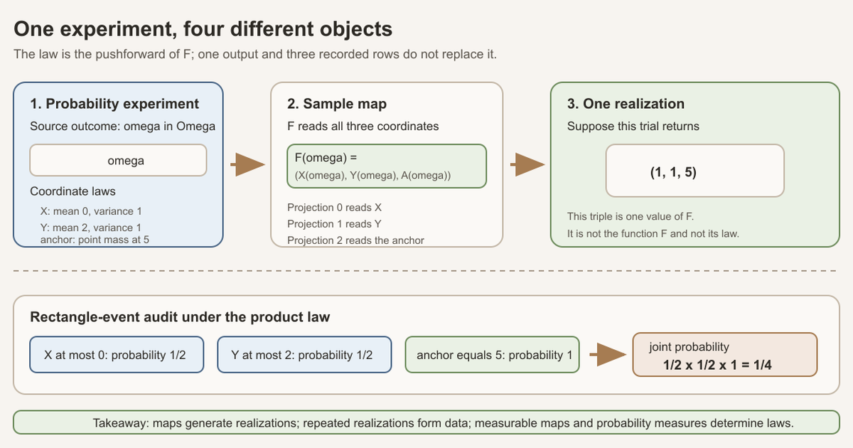
\[ F:\Omega\longrightarrow\mathbb R^3, \qquad F(\omega)=\bigl(X(\omega),Y(\omega),A(\omega)\bigr), \]where the three coordinate maps are mutually independent under a probability measure \(\mathbb P\), and their exact laws are
\[ X\sim\gamma_{0,1}, \qquad Y\sim\gamma_{2,1}, \qquad A\sim\gamma_{5,0}=\delta_5. \]Here \(\gamma_{m,v}\) means the real Gaussian probability law with mean \(m\) and variance \(v\). The last coordinate has variance zero, so its law is the Dirac measure at 5. It is an exact deterministic anchor, apart from changes on a probability-zero set.
The joint law of the whole triple is
\[ \mathcal L_{\mathbb P}(F) =\gamma_{0,1}\otimes\gamma_{2,1}\otimes\delta_5. \]That one line contains four separate ingredients: three marginal laws and one dependence assertion. The marginals identify each coordinate distribution. Mutual independence is what turns them into the displayed product law.
One output is not the law
Suppose the chosen sample map \(F\), whose law is the displayed product measure, has some \(\omega_1\in\Omega\) satisfying
\[ F(\omega_1)=(1,1,5). \]This triple is a realization, one value returned by the map \(F\). It is not the map itself, and it is not the probability law of that map. The existence of this exact fiber is an additional hypothesis about the chosen sample map, not a consequence of the displayed law.
This joint law gives every singleton zero mass because its first Gaussian marginal is atomless, even though its third coordinate is fixed at \(5\). Some value in \(\mathbb R^3\) is returned at each outcome, but the law only says that the preimage of each preselected value has probability zero. That preimage may be empty or nonempty; the law does not distinguish those cases.
Now consider the following hypothetical three-value record. These rows are chosen for arithmetic illustration; the product law neither supplies nor guarantees this exact data set.
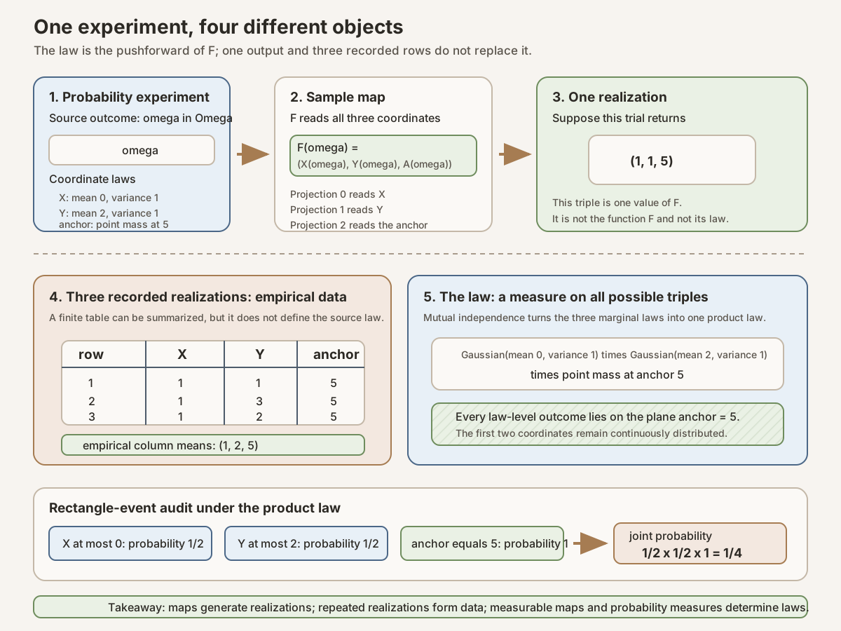
\[ (1,1,5),\qquad(1,3,5),\qquad(1,2,5). \]The empirical column means are \((1,2,5)\). The law-level mean vector is \((0,2,5)\). There is no contradiction. If the rows were an observed finite data table, their empirical mean would estimate the law-level mean; it would not redefine the law.
A product event can be computed exactly
Consider the measurable rectangle event
\[ E=\{X\le 0\}\cap\{Y\le 2\}\cap\{A=5\}. \]The first two thresholds sit at the means of symmetric nondegenerate Gaussians, so each has probability \(1/2\). The anchor event has probability
- Mutual independence gives
This calculation is exact. It is not estimated from the three rows above.
The five objects in the opening example
The vocabulary can now be attached to something concrete.
| Layer | Object in the example | What it answers |
|---|---|---|
| Probability base | \((\Omega,\mathcal F,\mathbb P)\) | Which outcomes exist, which events are measurable, and how much probability they receive |
| Sample map | \(F(\omega)=(X(\omega),Y(\omega),A(\omega))\) | Which triple is produced by each outcome |
| Realization | \(F(\omega_1)=(1,1,5)\) | What one particular outcome produced |
| Data | the three recorded rows | What a finite collection of trials produced |
| Law | \(F_*\mathbb P\) | How probability is distributed over all triples |
A random variable is a measurable map, not an automatically generated numeral. Its probability law is the pushforward measure
\[ \mathcal L_{\mathbb P}(F)=F_*\mathbb P. \]For a measurable set \(B\subseteq\mathbb R^3\), this means
\[ (F_*\mathbb P)(B) =\mathbb P\!\left(\{\omega:F(\omega)\in B\}\right). \]The pushforward forgets the private identity of the source outcomes while retaining the probability of every measurable value event. The event \(E\) above is the preimage of one rectangle in \(\mathbb R^3\).
The word distribution is often used for the law. A probability distribution is therefore a probability measure on the value space, not the three-row table. The table has an empirical distribution, a different measure constructed from observed values.
One exact real Gaussian law
For \(m\in\mathbb R\) and \(v\ge 0\), write \(\gamma_{m,v}\) for the real Gaussian measure with mean \(m\) and variance \(v\). When \(v\gt 0\), it has the familiar density
\[ f_{m,v}(x) =\frac{1}{\sqrt{2\pi v}} \exp\!\left(-\frac{(x-m)^2}{2v}\right). \]The mean \(m\) sets the center. The variance \(v\) measures expected squared distance from the center. The standard deviation is
\[ \sigma=\sqrt v. \]The NIST normal-distribution reference
uses a location parameter and a positive scale parameter in its density. In
this project and in Mathlib’s gaussianReal, the second explicit
parameter is variance, not standard deviation. That typing decision prevents
a silent square from appearing later.
Variance zero is the Dirac branch
The density formula cannot be used at \(v=0\), because its denominator would vanish. The probability measure itself still has a perfectly good boundary:
\[ \gamma_{m,0}=\delta_m. \]The Dirac measure \(\delta_m\) puts probability 1 at \(m\). In the running example, \(A\sim\delta_5\), so \(A=5\) almost everywhere. This is why the third coordinate of every displayed data row is 5 and why \(\mathbb P(A=5)=1\).
“Almost everywhere” is important. A function can be changed on a null set , an event of probability zero, without changing its law. Thus a law-level theorem gives
\[ A(\omega)=5\quad\text{for almost every }\omega, \]not necessarily a pointwise equation for every conceivable source outcome. The almost-everywhere relation records exactly this tolerance.
Lean bridge: an exact law is a pushforward claim
HasRealGaussianLaw X 0 (1 : ℝ≥0) PHasRealGaussianLawis the project’s exact, parameter-preserving proposition. A proof of this proposition is evidence about a law; it does not draw a sample.Xis a function from outcomes to real values.0is the mean parameter.(1 : ℝ≥0)is the variance. The type \(\mathbb R_{\ge0}\), calledNNRealin Lean, rules out negative variances.Pis the source measure, so the law statement never relies on an implicit default experiment.
The definition unfolds to
HasLaw X (gaussianReal 0 (1 : ℝ≥0)) P
where HasLaw combines almost-everywhere measurability with the
exact pushforward identity. The full project command that checks this
definition and all following project bridges appears in the final
repo-check. The local Std worksheet later in this
chapter checks only the finite ledger.
Measurability has two levels
A measurable function has measurable preimages of measurable sets. That is the condition that lets us assign probabilities to statements about its output.
Mathlib’s HasLaw X μ P stores
AEMeasurable X P, meaning that \(X\) agrees almost everywhere with an ordinarily measurable function; andMeasure.map X P = μ, the exact pushforward identity.
It does not silently upgrade \(X\) to Measurable X. This is
mathematically natural: changing a map on a null set does not change its law.
The project family structure nevertheless records ordinary coordinate
measurability separately, because later coordinate transformations and
product interfaces often need it directly.
This distinction can be hidden by paper notation. Lean makes it visible because
Measurable X and AEMeasurable X P are different types
of evidence.
Mean, variance, and standard deviation under scaling
If \(X\sim\gamma_{m,v}\) and \(c\in\mathbb R\), then
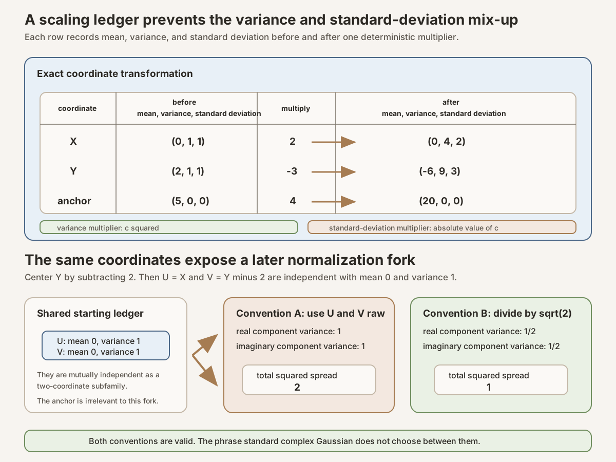
\[ cX\sim\gamma_{cm,c^2v}. \]The mean sees the signed multiplier \(c\). Variance sees its square \(c^2\). Standard deviation sees its absolute value \(|c|\):
\[ \operatorname{sd}(cX)=|c|\operatorname{sd}(X). \]Apply this to all three running coordinates:
| Coordinate | Before: mean, variance, standard deviation | Multiplier | After: mean, variance, standard deviation |
|---|---|---|---|
| \(X\) | \((0,1,1)\) | \(2\) | \((0,4,2)\) |
| \(Y\) | \((2,1,1)\) | \(-3\) | \((-6,9,3)\) |
| \(A\) | \((5,0,0)\) | \(4\) | \((20,0,0)\) |
The negative multiplier reverses the mean of \(Y\), but spread is nonnegative. The deterministic anchor remains deterministic. Scaling the anchor by zero would produce \(\delta_0\), another reason not to exclude the zero-variance branch.
Lean bridge: zero variance means almost-everywhere constancy
HasRealGaussianLaw A 5 0 P ↔ A =ᵐ[P] fun _ ↦ 5↔is logical equivalence: both directions are proved.=ᵐ[P]is equality almost everywhere with respect toP, not pointwise function equality.fun _ ↦ 5is the constant function returning 5 on every outcome.- The theorem is named
HasRealGaussianLaw.zero_variance_iffand assumes[IsProbabilityMeasure P].
The corresponding one-way theorem
ae_eq_const_of_variance_zero can obtain the probability-measure
instance from the exact law itself. Both belong to the full project module
checked by the repository command below.
Lean bridge: the type displays the square
HasRealGaussianLaw (fun ω ↦ c * X ω) (c * m) (⟨c ^ 2, sq_nonneg c⟩ * v) Pfun ω ↦ c * X ωis the transformed sample map.c * mis the transformed mean.c ^ 2is the real square.sq_nonneg cis Lean’s proof that this square is nonnegative.⟨c ^ 2, sq_nonneg c⟩packages the real number and its proof as anNNRealbefore multiplying byv.
The theorem is HasRealGaussianLaw.const_mul. The square is visible
in the conclusion, so a reader cannot accidentally interpret the input
variance as a standard deviation. Replay the exact theorem with the Full
project command in the repository check; replay the numeric table with
the standalone worksheet.
Marginals do not determine a joint law
The marginal law of \(X\) tells us the probabilities of events depending only on \(X\). It says nothing by itself about how \(X\) moves with \(Y\).
Here is a concrete near-miss. Let \(G\sim\gamma_{0,1}\).
- In one experiment, take \(X=G\) and let \(Y\sim\gamma_{2,1}\) be independent of \(G\).
- In another experiment, take \(X=G\) and set \(Y=G+2\).
Both experiments have the same two marginal laws:
\[ X\sim\gamma_{0,1},\qquad Y\sim\gamma_{2,1}. \]Their joint laws are radically different. In the second experiment every output lies on the line \(y=x+2\). Once \(X\) is known, \(Y\) is known. In the first experiment the joint law spreads across the plane and factors as a product. Thus the notation
\[ X\sim\gamma_{0,1},\qquad Y\sim\gamma_{2,1} \]does not entitle us to write
\[ (X,Y)\sim\gamma_{0,1}\otimes\gamma_{2,1}. \]The missing hypothesis is independence.
Pairwise independence is not mutual independence
For two random variables, independence means that every measurable event about the first factors from every measurable event about the second. For an indexed family, mutual independence requires the analogous factorization for every finite selection of distinct coordinates and measurable coordinate events.
Pairwise independence checks only two coordinates at a time. Those checks can all pass while a higher-order constraint remains.
Take two fair bits \(B_1,B_2\) and define the third bit by exclusive-or, \(B_3=B_1\mathbin{\mathrm{xor}}B_2\). The four equally likely triples are
\[ (0,0,0),\quad(0,1,1),\quad(1,0,1),\quad(1,1,0). \]Each bit is fair. Every pair displays all four pair values once, so every pair is independent. Yet
\[ \mathbb P(B_1=0,B_2=0,B_3=0)=\frac14, \]while mutual independence would require
\[ \mathbb P(B_1=0)\mathbb P(B_2=0)\mathbb P(B_3=0)=\frac18. \]The parity relation is invisible to every pair test.
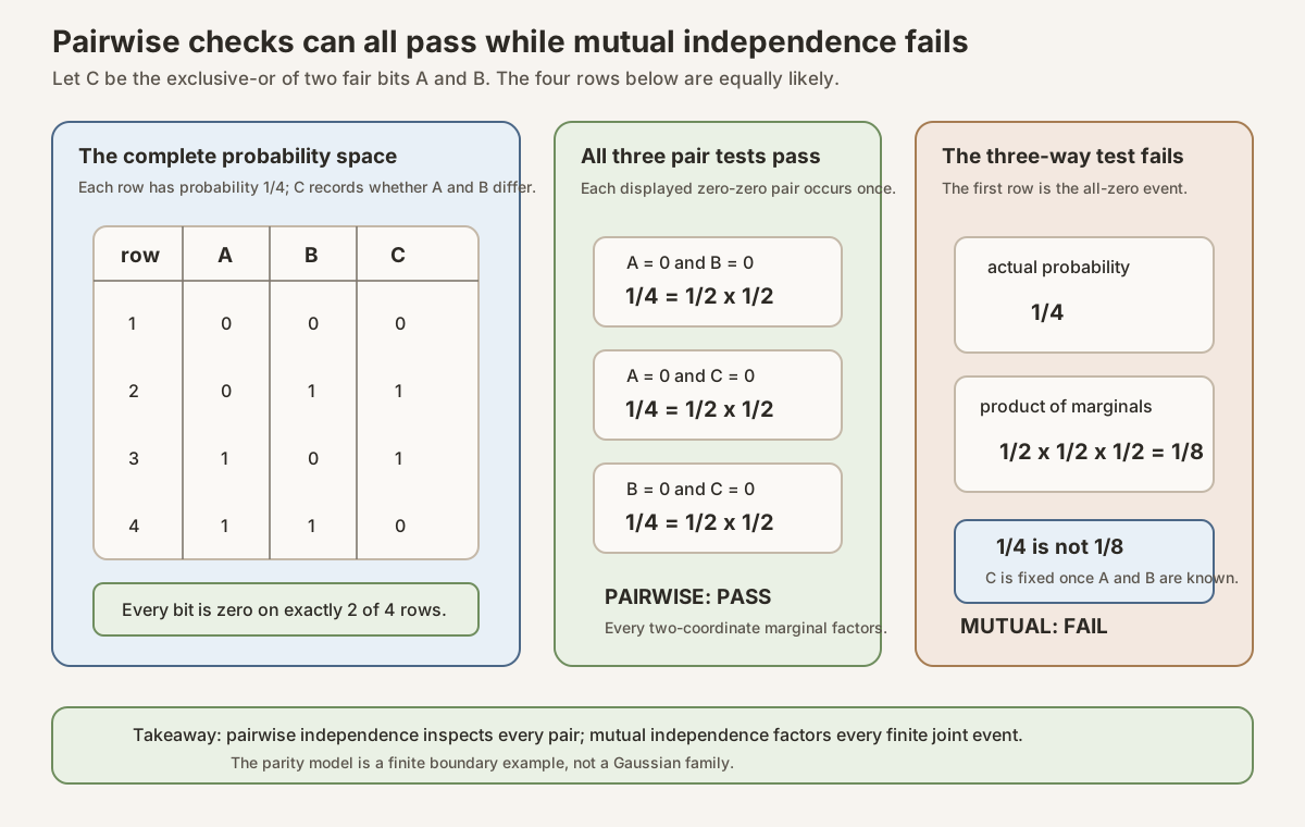
The example is deliberately not Gaussian. It is a counterexample to the universal implication from pairwise independence to mutual independence: “every pair is independent” and “the family is mutually independent” are different statements. Scalar Gaussian marginals alone do not erase that difference. A separately defined jointly Gaussian vector has stronger structure, but that is not what a list of scalar law claims says.
Package the whole family, not three loose facts
For an index type \(I\), write
\[ X_i:\Omega\to\mathbb R, \qquad m_i\in\mathbb R, \qquad v_i\in\mathbb R_{\ge0}. \]The project’s IndependentRealGaussianFamily structure stores
three fields:
- every coordinate map \(X_i\) is ordinarily measurable;
- every coordinate has the exact law \(\gamma_{m_i,v_i}\); and
- the complete coordinate family is mutually independent.
The index type may be infinite at this stage. Finiteness is introduced only when a finite product law is requested.
Lean bridge: three fields make the contract explicit
IndependentRealGaussianFamily X m v PThe structure is constructed from these exact fields:
structure IndependentRealGaussianFamily
    (X : ι → Ω → ℝ) (m : ι → ℝ) (v : ι → ℝ≥0)
    (P : Measure Ω) : Prop where
  measurable : ∀ i, Measurable (X i)
  hasLaw : ∀ i, HasRealGaussianLaw (X i) (m i) (v i) P
  independent : iIndepFun X P
ι → Ω → ℝis an indexed collection of real sample maps.mandvare parameter ledgers indexed by the same type, so every coordinate keeps its own mean and variance.∀ imeans “for every index.”iIndepFun X Pis Mathlib’s mutual-independence predicate for the whole family underP.- Ordinary measurability is a separate field because the exact law supplies only almost-everywhere measurability.
The exact source is checked by the full project command near the end. The
standalone local worksheet mirrors the three-coordinate parameter ledger but
does not implement Measure, HasLaw, or
iIndepFun.
Mutual independence produces the finite product law
Now assume \(I\) is finite. Bundle all coordinates into one map
\[ \mathbf X:\Omega\to(I\to\mathbb R), \qquad \mathbf X(\omega)(i)=X_i(\omega). \]This notation treats an \(I\)-indexed vector as a function from indices to values. For the running three-coordinate example, evaluating at the three indices retrieves \(X\), \(Y\), and \(A\).
The exact joint law is
\[ \mathcal L_{\mathbb P}(\mathbf X) =\bigotimes_{i\in I}\gamma_{m_i,v_i}. \]For a measurable rectangle \(\prod_i B_i\), product structure says
\[ \mathbb P\!\left(\bigcap_{i\in I}\{X_i\in B_i\}\right) =\prod_{i\in I}\gamma_{m_i,v_i}(B_i). \]The opening \(1/4\) computation is one instance, with
\[ B_X=(-\infty,0],\qquad B_Y=(-\infty,2],\qquad B_A=\{5\}. \]The Mathlib finite product-measure API constructs this measure on the function space and proves its rectangle factorization properties.
Lean bridge: the joint map has a product measure as its law
HasLaw (fun ω i ↦ X i ω) (Measure.pi fun i ↦ gaussianReal (m i) (v i)) Pfun ω i ↦ X i ωis a curried function: give it an outcome and then an index to retrieve that coordinate.Measure.piconstructs the finite product measure onι → ℝ.fun i ↦ gaussianReal (m i) (v i)supplies the marginal measure at indexi.HasLawidentifies the entire pushforward law, not merely its means, variances, or rectangle probabilities.
The project theorem is
IndependentRealGaussianFamily.jointHasLaw. It requires
[Fintype ι] at exactly this product step. The same full project
module also proves jointHasGaussianLaw, which forgets the explicit
parameter ledger and retains qualitative joint Gaussianity.
Independence also explains sums
If \(X\sim\gamma_{m_X,v_X}\) and \(Y\sim\gamma_{m_Y,v_Y}\) are independent, then
\[ X+Y\sim\gamma_{m_X+m_Y,v_X+v_Y}. \]For the running pair,
\[ X+Y\sim\gamma_{2,2}. \]The variance is 2, so the standard deviation is \(\sqrt2\), not 2. Without
independence, a covariance term may change the variance of the sum. The exact
project theorem therefore accepts an explicit IndepFun X Y P
hypothesis rather than inferring it from the two scalar law proofs.
A canonical product experiment exists
An abstract family may live on a complicated source space \(\Omega\). For a finite index type \(I\), there is also a canonical choice:
\[ \Omega_{\mathrm{can}}=I\to\mathbb R, \qquad \mathbb P_{\mathrm{can}} =\bigotimes_{i\in I}\gamma_{m_i,v_i}. \]An outcome \(x\in I\to\mathbb R\) is already a complete coordinate tuple. The \(i\)-th random variable is just evaluation,
\[ \pi_i(x)=x(i). \]Under the product measure, these evaluation maps have the requested marginal laws and are mutually independent. This is more than saying that such random variables “should exist.” It gives one explicit probability space that later constructions can reuse.
Lean bridge: projections are the canonical independent family
gaussianProductMeasure_independentFamily m vThe supporting definition and the two component theorems are
gaussianProductMeasure m v
gaussianProductMeasure_hasLaw_eval m v i
gaussianProductMeasure_iIndepFun m v
gaussianProductMeasure m vabbreviatesMeasure.pi fun i ↦ gaussianReal (m i) (v i).fun x : ι → ℝ ↦ x iis the coordinate projection.measurable_pi_apply iproves ordinary measurability of that projection.gaussianProductMeasure_independentFamily m vpackages measurability, exact laws, and mutual independence into the family structure.
For an empty finite index type, the function space has one empty tuple and the product measure is Dirac at that tuple. This is a scalar product-space policy. It does not decide any later zero-dimensional matrix-ensemble convention. Use the full project check to elaborate these exact Mathlib-dependent declarations.
Type and run the finite ledger yourself
The measure-theoretic declarations above import Mathlib and are full project
checks that may require substantial disk space and memory. The finite
arithmetic and type distinctions from the opening example form a standalone
tutorial for an ordinary macOS or Linux machine. This worksheet imports only
Lean’s Std library.
Open a text editor, create /tmp/GaussianFamilyTutorial.lean, and
type the following code. Typing it matters: each definition makes one layer
of the example explicit.
import Std

inductive Coord where
  | x
  | y
  | anchor
deriving Repr, DecidableEq

def coords : List Coord := [.x, .y, .anchor]

def coordLabel : Coord → String
  | .x => "X"
  | .y => "Y"
  | .anchor => "anchor"

structure LawParams where
  mean : Int
  variance : Int
  stdDev : Int
deriving Repr, DecidableEq

def lawParams : Coord → LawParams
  | .x => ⟨0, 1, 1⟩
  | .y => ⟨2, 1, 1⟩
  | .anchor => ⟨5, 0, 0⟩

def scaleCoefficient : Coord → Int
  | .x => 2
  | .y => -3
  | .anchor => 4

def absInt (z : Int) : Int :=
  if z < 0 then -z else z

def scaleParams (c : Int) (p : LawParams) : LawParams :=
  ⟨c * p.mean, c * c * p.variance, absInt c * p.stdDev⟩

def paramsConsistent (p : LawParams) : Bool :=
  decide (p.variance = p.stdDev * p.stdDev ∧
    0 ≤ p.variance ∧ 0 ≤ p.stdDev)

structure Observation where
  x : Int
  y : Int
  anchor : Int
deriving Repr, DecidableEq

def observationEntries (row : Observation) : Int × Int × Int :=
  (row.x, row.y, row.anchor)

def observations : List Observation :=
  [⟨1, 1, 5⟩, ⟨1, 3, 5⟩, ⟨1, 2, 5⟩]

def addObservation (left right : Observation) : Observation :=
  ⟨left.x + right.x, left.y + right.y, left.anchor + right.anchor⟩

def columnSums : Observation :=
  observations.foldl addObservation ⟨0, 0, 0⟩

def empiricalMeans : Observation :=
  let n : Int := observations.length
  ⟨columnSums.x / n, columnSums.y / n, columnSums.anchor / n⟩

def eventNumeratorsInEighths : List (String × Nat) :=
  [("X <= 0", 4), ("Y <= 2", 4), ("anchor = 5", 8)]

def productEventNumeratorInEighths : Nat :=
  (4 * 4 * 8) / (8 * 8)

structure BitTriple where
  a : Bool
  b : Bool
  c : Bool
deriving Repr, DecidableEq

def parityRows : List BitTriple :=
  [⟨false, false, false⟩, ⟨false, true, true⟩,
   ⟨true, false, true⟩, ⟨true, true, false⟩]

def countRows (predicate : BitTriple → Bool) : Nat :=
  parityRows.foldl (fun total row =>
    if predicate row then total + 1 else total) 0

def pairZeroCounts : List Nat :=
  [countRows (fun row => !row.a && !row.b),
   countRows (fun row => !row.a && !row.c),
   countRows (fun row => !row.b && !row.c)]

def tripleZeroCount : Nat :=
  countRows (fun row => !row.a && !row.b && !row.c)

def actualTripleProbabilityInEighths : Nat := tripleZeroCount * 2
def mutualProductProbabilityInEighths : Nat := 1

#eval coords.map (fun i =>
  (coordLabel i, (lawParams i).mean, (lawParams i).variance,
    (lawParams i).stdDev))
#eval observations.map observationEntries
#eval observationEntries empiricalMeans
#eval coords.map (fun i =>
  let p := scaleParams (scaleCoefficient i) (lawParams i)
  (coordLabel i, p.mean, p.variance, p.stdDev))
#eval coords.all (fun i =>
  paramsConsistent (scaleParams (scaleCoefficient i) (lawParams i)))
#eval (eventNumeratorsInEighths, productEventNumeratorInEighths)
#eval (pairZeroCounts, actualTripleProbabilityInEighths,
  mutualProductProbabilityInEighths)

example : observationEntries empiricalMeans = (1, 2, 5) := by
  native_decide

example :
    coords.map (fun i =>
      let p := scaleParams (scaleCoefficient i) (lawParams i)
      (p.mean, p.variance, p.stdDev)) =
      [(0, 4, 2), (-6, 9, 3), (20, 0, 0)] := by
  native_decide

example : productEventNumeratorInEighths = 2 := by
  native_decide

example : pairZeroCounts = [1, 1, 1] := by
  native_decide

example :
    actualTripleProbabilityInEighths = 2 ∧
      mutualProductProbabilityInEighths = 1 := by
  native_decide
With Elan installed, run the exact pinned Lean release:
source "$HOME/.elan/env"
elan run leanprover/lean4:v4.32.0 lean /tmp/GaussianFamilyTutorial.lean
Resource label: small standalone Lean plus Std, suitable for a
normal Mac or Linux machine. This command does not enter the repository’s
Lake project and does not build Mathlib.
The worksheet was executed with that command and printed:
[("X", 0, 1, 1), ("Y", 2, 1, 1), ("anchor", 5, 0, 0)]
[(1, 1, 5), (1, 3, 5), (1, 2, 5)]
(1, 2, 5)
[("X", 0, 4, 2), ("Y", -6, 9, 3), ("anchor", 20, 0, 0)]
true
([("X <= 0", 4), ("Y <= 2", 4), ("anchor = 5", 8)], 2)
([1, 1, 1], 2, 1)
Read those lines as a ledger:
- the exact parameter table keeps mean, variance, and standard deviation in separate fields;
- the next two lines separate observed rows from their empirical means;
- the scaled table confirms the three numeric transformations;
trueconfirms variance equals standard deviation squared in every scaled row;- probabilities are stored in eighths, so the rectangle numerator 2 means \(2/8=1/4\); and
- every zero-zero pair occurs once in four parity rows, while the all-zero triple is \(2/8=1/4\), not the mutual-product value \(1/8\).
The five example blocks are propositions checked by Lean’s kernel.
They verify finite lists and integer arithmetic. They do not define a
Gaussian measure, prove a density integral, establish independence of real
random variables, or check the Mathlib-dependent project module. Those claims
belong to the next resource layer.
Inspect the checked project interfaces
The authoritative source is
formalization/NonlinearDynamics/Random/GaussianPrimitives.lean.
It imports the pinned Mathlib Gaussian and independence APIs. Type the probe
below into a temporary project scratch file after installing the repository’s
pinned dependencies.
Full project check: exact repository module plus Mathlib. The following probe requests the types of the declarations used throughout the chapter:
import NonlinearDynamics.Random.GaussianPrimitives

open MeasureTheory ProbabilityTheory
open scoped ENNReal NNReal ProbabilityTheory
open NonlinearDynamics.Random

#check HasRealGaussianLaw
#check HasRealGaussianLaw.mean_eq
#check HasRealGaussianLaw.variance_eq
#check HasRealGaussianLaw.zero_variance_iff
#check HasRealGaussianLaw.const_mul
#check HasRealGaussianLaw.add_of_indep
#check IndependentRealGaussianFamily
#check IndependentRealGaussianFamily.scale
#check IndependentRealGaussianFamily.jointHasLaw
#check IndependentRealGaussianFamily.jointHasGaussianLaw
#check gaussianProductMeasure
#check gaussianProductMeasure_hasLaw_eval
#check gaussianProductMeasure_iIndepFun
#check gaussianProductMeasure_independentFamily
import loads the exact project module. Each #check
elaborates an existing name and reports its type; it neither draws
samples nor proves a new theorem. The full project command rendered immediately
below checks the authoritative source file with the repository’s pinned
toolchain and dependencies.
cd formalization
lake env lean -DwarningAsError=true NonlinearDynamics/Random/GaussianPrimitives.lean
Resource note: this exact file uses the repository's
pinned Lean and Mathlib dependencies. Initial project setup can require
substantial disk space and build time. For a lightweight first step on
macOS or Linux, use the page's standalone Lean-core or Std
tutorial.
What the checked module proves
The source file contains no sorry or admit. Its public
surface can be read as a dependency ladder.
| Declaration | Checked content | It does not claim |
|---|---|---|
HasRealGaussianLaw | exact real Gaussian pushforward law with explicit mean and variance | that one observed value or histogram is Gaussian |
aemeasurable | almost-everywhere measurability from the exact law | ordinary measurability |
isProbabilityMeasure | the source measure is a probability measure | independence from another variable |
mean_eq | the integral of the variable equals its mean parameter | a sample mean identity |
variance_eq | Mathlib variance equals the variance parameter | that variance and standard deviation are the same |
hasGaussianLaw | forgets explicit parameters and retains qualitative Gaussianity | recovery of a chosen parameter pair |
memLp, integrable | finite-moment and integrability consequences | a matrix observable or spectral moment |
ae_eq_const_of_variance_zero | zero variance gives almost-everywhere constancy | pointwise equality on null-set modifications |
zero_variance_iff | under a probability measure, the Dirac law and almost-everywhere constancy are equivalent | a positive-variance density formula at zero |
const_mul | real scaling transforms mean and variance exactly | a choice of complex normalization |
add_of_indep | independent Gaussian sums add means and variances | the same law without independence |
IndependentRealGaussianFamily | ordinary measurability, exact marginal laws, and mutual independence | finiteness of the index type |
scale | coordinatewise deterministic scaling preserves the family contract | nonlinear transformations staying Gaussian |
jointHasLaw | a finite family’s vector law is the product of its marginal Gaussian measures | that marginals alone imply the product law |
jointHasGaussianLaw | the finite vector is qualitatively jointly Gaussian | retention of the explicit parameter ledger in that predicate |
gaussianProductMeasure | canonical finite product probability measure | a complex or matrix ensemble |
| projection theorems | exact projection laws, mutual independence, and the packaged canonical family | a sampling algorithm or pseudorandom generator |
The Mathlib real Gaussian documentation, law API, and independence API are the upstream implementation references for this layer.
The normalization question remains open here
Return to the two nondegenerate coordinates. Center the second one:
\[ U=X, \qquad V=Y-2. \]Then \(U\) and \(V\) are independent, centered, real Gaussians with variance
- They can be used to form a complex variable in at least two common ways:
For the raw choice,
\[ \operatorname{Var}(\operatorname{Re}Z_{\mathrm{raw}})=1, \qquad \operatorname{Var}(\operatorname{Im}Z_{\mathrm{raw}})=1, \qquad \mathbb E|Z_{\mathrm{raw}}|^2=2. \]For the divided choice,
\[ \operatorname{Var}(\operatorname{Re}Z_{\mathrm{unit}})=\frac12, \qquad \operatorname{Var}(\operatorname{Im}Z_{\mathrm{unit}})=\frac12, \qquad \mathbb E|Z_{\mathrm{unit}}|^2=1. \]Both constructions are mathematically valid. The phrase “standard complex Gaussian” does not by itself say whether “standard” refers to each real component or to the total centered squared magnitude. A formal development must record the convention as data or a definition before proving downstream matrix formulas.
That is why the module in this chapter deliberately stops at real Gaussian
primitives. It proves neither a complex Gaussian law nor a matrix ensemble.
The later
Complex Gaussian Coordinates and Geometry
chapter describes the repository’s subsequent explicit two-component choice.
The later existence of that module does not retroactively put a normalization
choice inside GaussianPrimitives.
Why matrix normalization needs an even larger ledger
A Hermitian random matrix adds several choices:
| Ledger slot | Question that must be answered |
|---|---|
| Dimension | What is the index type and what happens at size zero? |
| Diagonal coordinates | What exact real means and variances are used? |
| Upper coordinates | What are the real and imaginary component variances? |
| Dependence | Which primitive coordinates are mutually independent? |
| Reflection | How are lower entries obtained from upper entries? |
| Dimension scaling | Is an entry divided by \(\sqrt n\), \(\sqrt{2n}\), or something else? |
| Trace | Is the observable \(\operatorname{tr}\) or \(n^{-1}\operatorname{tr}\)? |
| Density | Which reference volume and exponent coefficient are intended? |
| Spectral scale | At what magnitude should eigenvalues live? |
An entrywise construction, a density on Hermitian matrices, and a symmetry-based characterization may eventually describe the same law. Their equivalence is a theorem, not something supplied by the word “Gaussian.” Dyson’s symmetry-class work motivates why these distinctions matter in quantum spectral models, but it does not choose this project’s numerical normalization.
Common wrong turns
| Wrong turn | Why it fails | Correct repair |
|---|---|---|
| “The three rows look plausible, so the law is Gaussian.” | A finite data set is not an exact pushforward law. | Separate statistical evidence from HasLaw. |
| “The empirical mean is 1, so the first law mean cannot be 0.” | A sample mean is random and need not equal the law mean. | Keep data summaries and distribution parameters in different layers. |
| “All coordinates are Gaussian, so the vector law is a product.” | Marginal laws do not contain dependence information. | Add mutual independence. |
| “Every pair is independent, so the family is independent.” | A higher-order constraint can survive all pair checks. | Use a mutual-family predicate such as iIndepFun. |
| “Variance one means standard deviation one, so the words are interchangeable.” | They coincide numerically only at 1 and obey different scaling rules. | Record both columns and square the scale for variance. |
| “Variance zero breaks the Gaussian definition.” | Only the positive-variance density breaks; the measure becomes Dirac. | Define the degenerate measure branch. |
| “Dirac law means pointwise constant.” | Law ignores changes on null sets. | State almost-everywhere equality. |
“HasLaw proves ordinary measurability.” | Its field is almost-everywhere measurability. | Store Measurable separately when needed. |
| “A list of means and variances identifies the joint law.” | Moments do not determine dependence in general. | Prove the complete pushforward or product law. |
| “Standard complex Gaussian has one universal scale.” | Component and total-spread conventions differ. | Fill the normalization ledger explicitly. |
| “The standalone worksheet checked the Gaussian theorem.” | It checked finite integer bookkeeping only. | Run the exact Mathlib/project declaration as a full project check. |
Exercises: keep using the same coordinates
- Objects. For the value \((1,3,5)\), identify the map, outcome-dependent realization, data row, and law. Explain why none can replace another.
- Empirical law. Write the empirical measure of the three rows as a sum of three Dirac measures with weights \(1/3\). What mass does it assign to the plane \(a=5\)?
- Rectangle. Replace \(Y\le2\) by \(Y\gt2\). Compute the product-event probability using symmetry.
- Degenerate branch. Replace the anchor mean 5 by \(-4\). State its law, almost-everywhere equality, and probability of the event \(A=-4\).
- Scaling. Multiply \(X\) by \(-5\). Record its new mean, variance, and standard deviation before changing the worksheet.
- Translation. Center \(Y\) by subtracting 2. Which law does \(Y-2\) have? Which parameter changes and which does not?
- Sum. Compute the law of \(2X-3Y\) using mutual independence. Keep mean, variance, and standard deviation separate.
- Marginal near-miss. For the coupled construction \(Y=X+2\), calculate the probability of the event \(Y=X+2\). Compare it with the independent product experiment.
- Parity. List the four values of each pair \((B_1,B_2)\), \((B_1,B_3)\), and \((B_2,B_3)\). Then test one three-way event other than the all-zero event.
- Lean tokens. In the standalone worksheet, change the anchor mean to \(-4\) and its scale coefficient to zero. Update the displayed output and all affected examples.
- Canonical space. For three named indices, explain why one canonical outcome is a function from those indices to \(\mathbb R\), even if it is written informally as a triple.
- Empty index. How many functions exist from the empty type to \(\mathbb R\)? Why is a Dirac measure at that unique function the natural empty product?
- Normalization. Derive the component variances and total squared spread of \((U+iV)/2\). Which familiar convention, if either, does it match?
- Resource boundary. Explain why the standalone tutorial is small while the full project probe loads the repository’s pinned Mathlib dependencies.
- Research boundary. Name three additional declarations required before an exact real product family becomes a unitary-invariant random matrix law.
Summit summary
The running example now supports the entire dependency chain:
\[ \begin{aligned} &\text{probability base} \longrightarrow \text{measurable coordinate maps} \longrightarrow \text{realizations and data},\\ &\text{exact marginal laws}+\text{mutual independence} \longrightarrow \text{joint product law},\\ &\text{exact means and variances} \longrightarrow \text{safe scaling and degeneracy rules},\\ &\text{real Gaussian primitives} \longrightarrow \text{an explicit, still unresolved complex normalization ledger}. \end{aligned} \]The layer contract is: never ask one layer to supply information that belongs to another. A realization does not supply a law. Marginals do not supply dependence. Pairwise checks do not supply mutual independence. Variance does not mean standard deviation. A density formula does not cover its degenerate boundary. The word “standard” does not supply a normalization.
Where to continue
- Gaussian distribution develops the scalar density, measure, and degenerate branch.
- Variance separates moments, variance, and standard deviation.
- Independence develops event factorization and indexed families.
- Probability law revisits maps, pushforwards, and samples.
- Normalization convention provides the broader complex and matrix ledger.
- Continue next to Complex Gaussian Coordinates and Geometry for the explicit Cartesian complex law.
- Then read Finite Product Probability Spaces and Independent Gaussian Fields for the next product-space layer.
- Finite GUE from Independent Gaussian Coordinates shows where a specified dimension-dependent matrix normalization is finally selected.
References
National Institute of Standards and Technology. Normal Distribution, Engineering Statistics Handbook. This official reference gives the positive-variance normal density and identifies its location and scale parameters.
Mathlib contributors.
Gaussian distributions over the reals,
Mathlib 4 documentation. This is the implementation-level reference for
gaussianReal, the zero-variance Dirac branch, probability status,
mean, variance, moments, scaling, convolution, and independent sums.
Mathlib contributors.
Law of a random variable,
Mathlib 4 documentation. This documents the
AEMeasurable and pushforward fields of HasLaw and the
law-transport interfaces used by the project.
Mathlib contributors.
Independence of functions,
Mathlib 4 documentation. This is the official reference for
IndepFun, iIndepFun, composition, and finite joint-law
factorization.
Mathlib contributors.
Finite product measures,
Mathlib 4 documentation. This documents Measure.pi, its
probability instance, coordinate evaluation laws, and measurable-rectangle
factorization.
Mathlib contributors. Gaussian laws and independence, Mathlib 4 documentation. This official source supports the qualitative joint Gaussian theorem used after the exact parameterized product-law theorem.
Freeman J. Dyson. Statistical Theory of the Energy Levels of Complex Systems. I, Journal of Mathematical Physics 3 (1962), 140–156. This primary historical source motivates symmetry-based matrix ensembles. It is not used to infer or approve this project’s normalization.
The exact upstream source audited for this chapter is Mathlib commit
81a5d257,
the revision recorded in formalization/lake-manifest.json.