Start with three states and multiply everything
Let the base state be one of
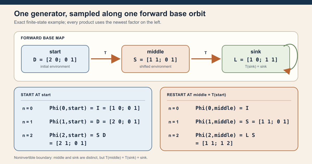
\[ \Omega=\{\mathsf{start},\mathsf{middle},\mathsf{sink}\}. \]One application of the base map \(T\) advances the environment:
\[ T(\mathsf{start})=\mathsf{middle}, \qquad T(\mathsf{middle})=\mathsf{sink}, \qquad T(\mathsf{sink})=\mathsf{sink}. \]This map is not invertible. The distinct states \(\mathsf{middle}\) and \(\mathsf{sink}\) have the same image. Forward iteration still makes perfect sense: from \(\mathsf{start}\) the orbit is
\[ \mathsf{start},\ \mathsf{middle},\ \mathsf{sink},\ \mathsf{sink},\ldots. \]Attach one integer \(2\)-by-\(2\) matrix to each state:
\[ \begin{aligned} A(\mathsf{start})=D&= \begin{bmatrix}2&0\\0&1\end{bmatrix},\\ A(\mathsf{middle})=S&= \begin{bmatrix}1&1\\0&1\end{bmatrix},\\ A(\mathsf{sink})=L&= \begin{bmatrix}1&0\\1&1\end{bmatrix}. \end{aligned} \]The letter \(A\) names one generator: a function from the current environment to a matrix. It is not a new unrelated function at each time. Time dependence comes from evaluating the same \(A\) after repeated applications of \(T\).
At horizon zero, no matrix has acted, so the value is the identity. At horizon one, use the matrix at the starting state. At horizon two, first \(D\) acts, the base moves to \(\mathsf{middle}\), and then \(S\) acts. With column vectors, the second action is written on the left:
\[ \begin{aligned} \Phi(0,\mathsf{start}) &=I=\begin{bmatrix}1&0\\0&1\end{bmatrix},\\ \Phi(1,\mathsf{start}) &=D=\begin{bmatrix}2&0\\0&1\end{bmatrix},\\ \Phi(2,\mathsf{start}) &=SD {} = \begin{bmatrix}1&1\\0&1\end{bmatrix} \begin{bmatrix}2&0\\0&1\end{bmatrix} {} = \begin{bmatrix}2&1\\0&1\end{bmatrix}. \end{aligned} \]Now restart the same calculation at the shifted point \(\mathsf{middle}=T(\mathsf{start})\). The next state is \(\mathsf{sink}\), so
\[ \begin{aligned} \Phi(0,\mathsf{middle})&=I,\\ \Phi(1,\mathsf{middle})&=S =\begin{bmatrix}1&1\\0&1\end{bmatrix},\\ \Phi(2,\mathsf{middle})&=LS {} = \begin{bmatrix}1&0\\1&1\end{bmatrix} \begin{bmatrix}1&1\\0&1\end{bmatrix} {} = \begin{bmatrix}1&1\\1&2\end{bmatrix}. \end{aligned} \]Every entry is now visible. The abstract definition later in the chapter is just this ledger with arbitrary states, horizons, and matrices.
Name the five objects before climbing
| Object | Running example | General notation |
|---|---|---|
| Base state | \(\mathsf{start}\) | \(\omega\in\Omega\) |
| Base map | start \(\mapsto\) middle \(\mapsto\) sink | \(T:\Omega\to\Omega\) |
| Generator | \(D,S,L\) selected by state | \(A:\Omega\to M_\iota(\mathbb K)\) |
| Orbit factor at time \(j\) | \(D,S,L,L,\ldots\) | \(A(T^j\omega)\) |
| Finite cocycle value | \(SD\) at horizon two from start | \(\Phi(j,\omega)\) |
The word random in the project namespace does not alter this calculation. A matrix-valued random variable is first of all a measurable function of an outcome. A probability measure or probability distribution is extra data. The unbundled algebra below does not use a measure at all.
If we equip this finite set with its full discrete measurable structure and later want the base inside the bundled measure-preserving interface, one possible measure is the Dirac mass \(\delta_{\mathsf{sink}}\). Because \(T(\mathsf{sink})=\mathsf{sink}\), that measure is preserved. This observation does not make the three displayed matrices independent or identically distributed, and the present Lean module does not define their pushforward laws.
Choose a route up
| Route | Begin with | Destination |
|---|---|---|
| First encounter | Start with three states | Compute horizons zero, one, and two at two base points |
| Iteration route | Natural-number iteration builds the orbit | Read Mathlib’s function-iterate notation and laws |
| Algebra route | One generator becomes a finite product | Derive zero, one, successor, and addition identities |
| Proof route | Why the cocycle proof needs an iterate calculation | Audit the induction and later-block-left order |
| Measure route | What measure preserving means | Separate invariance of a measure from probability and ergodicity |
| Hands-on Lean route | Type the example with Lean and Std | Run a bounded worksheet on an ordinary Mac or Linux machine |
| Lean route | The complete declaration map | Audit all sixteen names and their exact assumptions |
| Boundary route | Empty matrix dimension remains valid | See which declarations do not need finite nonempty coordinates |
| Summit route | What has and has not been proved | Preserve every explicit nonclaim |
Learning objectives
By the summit, you should be able to:
- distinguish a base state, base map, generator, orbit factor, and cocycle value;
- read
T^[j]as the \(j\)-fold natural-number iterate of \(T\); - explain why the orbit sequence itself needs no matrix algebra;
- reproduce the exact horizon-zero, one, and two ledgers from start and middle;
- explain why the newest factor is written on the left;
- derive the shifted later-block-left cocycle identity;
- identify where
Function.iterate_add_applyenters its proof; - distinguish a generator-presented cocycle from an axiom-presented one;
- separate semiring algebra from complex measurability;
- prove that each orbit factor is measurable by composition;
- define
MeasurePreservingas measurability plus pushforward equality; - explain why a measure-preserving base need not be probabilistic, ergodic, mixing, or invertible;
- explain why every natural-number base iterate preserves the measure;
- audit the exact four fields of
DiscreteMatrixCocycle; - run the pinned
Stdworksheet without loading Mathlib; - map every mathematical claim to one of the sixteen declarations;
- explain why empty matrix dimension is supported; and
- list the law, norm, integrability, asymptotic, and nonlinear-dynamics bridges still absent.
Base camp: natural-number iteration builds the orbit
For a self-map \(T:\Omega\to\Omega\), Mathlib’s
Function.iterate defines \(T^j\) for each natural number \(j\).
Lean writes this as T^[j].
The zeroth iterate is the identity:
\[ T^0\omega=\omega. \]The successor iterate applies \(T\) one more time:
\[ T^{j+1}\omega=T(T^j\omega). \]Iteration also adds:
\[ T^{m+k}\omega=T^k(T^m\omega) {} = T^m(T^k\omega). \]Both displayed forms are valid because they are iterates of the same map and natural-number addition commutes. This does not say that arbitrary functions commute.
The first declaration is:
def orbitMatrixSequence
    (T : Ω → Ω) (A : RandomMatrix Ω ι ι 𝕜) :
    ℕ → RandomMatrix Ω ι ι 𝕜 :=
  fun j ω => A (T^[j] ω)
In Lean: observe one generator after \(j\) base steps
fun j ω => A (T^[j] ω)fun j ω => …creates a function with two inputs: a natural timejand a base pointω.T^[j]is Lean notation for the \(j\)-fold iterate of the functionT. It is not a matrix power.T^[j] ωevaluates that iterated function atω.A (…)asks the same generator for the matrix at the reached state.- The exact project declaration is
orbitMatrixSequence. No multiplication, probability law, or independence statement occurs in this expression.
At time \(j\) and initial state \(\omega\), it returns
\(A(T^j\omega)\). This definition performs only evaluation and composition.
Its elaborated public type needs no Fintype ι, no decidable
equality, and no semiring on \(\mathbb K\). A matrix here is merely a
two-coordinate function.
That weak interface is useful. The orbit-generated sequence exists before any decision to multiply its values.
Camp one: read the first orbit factors
Fix \(\omega\). The first four factors are:
\[ \begin{array}{c|c|c} j & \text{base state} & \text{matrix factor}\\ \hline 0 & \omega & A(\omega)\\ 1 & T\omega & A(T\omega)\\ 2 & T^2\omega & A(T^2\omega)\\ 3 & T^3\omega & A(T^3\omega) \end{array} \]The initial state remains an argument. Changing \(\omega\) changes the entire forward orbit and can change every factor.
This sequence is a special case of the arbitrary time-indexed family from finite random-matrix products . The special feature is coherence across time: every factor comes from the same generator after a known base iterate.
No independence follows. Two factors \(A(T^j\omega)\) and \(A(T^\ell\omega)\) are functions of the same initial state and the same deterministic base map.
Camp two: one generator becomes a finite product
The definition
def cocycleProduct
    (T : Ω → Ω) (A : RandomMatrix Ω ι ι 𝕜) (k : ℕ) :
    RandomMatrix Ω ι ι 𝕜 :=
  MatrixProducts.sampleForwardProduct
    (orbitMatrixSequence T A) k
feeds the orbit sequence into the earlier pointwise product. This layer assumes that \(\iota\) is finite with decidable equality and that \(\mathbb K\) is a semiring.
The first product values are
\[ \begin{aligned} \Phi(0,\omega)&=I,\\ \Phi(1,\omega)&=A(\omega),\\ \Phi(2,\omega)&=A(T\omega)A(\omega),\\ \Phi(3,\omega)&=A(T^2\omega)A(T\omega)A(\omega). \end{aligned} \]The module exposes these facts through:
cocycleProduct_zero;cocycleProduct_succ; andcocycleProduct_one.
The zero and successor equations are definitional. The one-step theorem uses function extensionality and simplification to identify the sampled zeroth iterate with the original generator.
At a successor horizon,
\[ \Phi(k+1,\omega)=A(T^k\omega)\Phi(k,\omega). \]In Lean: append the newest factor on the left
cocycleProduct T A (k + 1) = fun ω => A (T^[k] ω) * cocycleProduct T A k ωk + 1is the successor horizon.fun ω =>states equality of the two matrix-valued functions by displaying their value at each base point.A (T^[k] ω)is the newest orbit factor.*is matrix multiplication here. Its left operand acts second on a column vector.cocycleProduct T A k ωis the already accumulated \(k\)-step value.- The exact theorem is
cocycleProduct_succ; its proof is definitional because the underlying forward product uses this recursion.
The newest factor is on the left. This convention is inherited from forward matrix products , not chosen again in the cocycle layer.
Camp three: why the cocycle proof needs an iterate calculation
The theorem cocycleProduct_add states, pointwise,
In Lean: split elapsed time and shift the later block
cocycleProduct T A (m + k) ω = cocycleProduct T A k (T^[m] ω) * cocycleProduct T A m ωm + kis the total forward horizon; both lengths are natural numbers.T^[m] ωis the split state reached by the early block.cocycleProduct T A k (T^[m] ω)recomputes the later block from that shifted point instead of from the original point.- The shifted \(k\)-block appears before
*, hence on the left. - The exact theorem is
cocycleProduct_add T A m k ω. It uses only semiring matrix algebra, not measurability or a measure.
Its proof inducts on the length \(k\) of the later block.
Later block of length zero
When \(k=0\), the later value is the identity:
\[ \Phi(m+0,\omega) {} = I\Phi(m,\omega). \]Simplification closes the base case.
Add one later step
Assume the theorem for \(k\). The newest factor on the full left side is
\[ A(T^{m+k}\omega). \]The newest factor in the shifted later product is
\[ A(T^k(T^m\omega)). \]These are equal by the iterate-addition law:
\[ T^{m+k}\omega=T^k(T^m\omega). \]Mathlib states Function.iterate_add_apply with a particular order
of the two natural indices. The Lean proof commutes \(m+k\) before applying
that theorem. This is an index normalization step, not a commutativity
assumption on matrices.
After the orbit states agree, the induction hypothesis replaces the shorter product, and matrix multiplication associativity closes the successor case. No factor is commuted across another.
The proof therefore uses exactly three structural ingredients:
- the successor recursion for the ordered product;
- addition of iterates of one base map; and
- associativity of matrix multiplication.
Camp four: audit the identity and two near misses
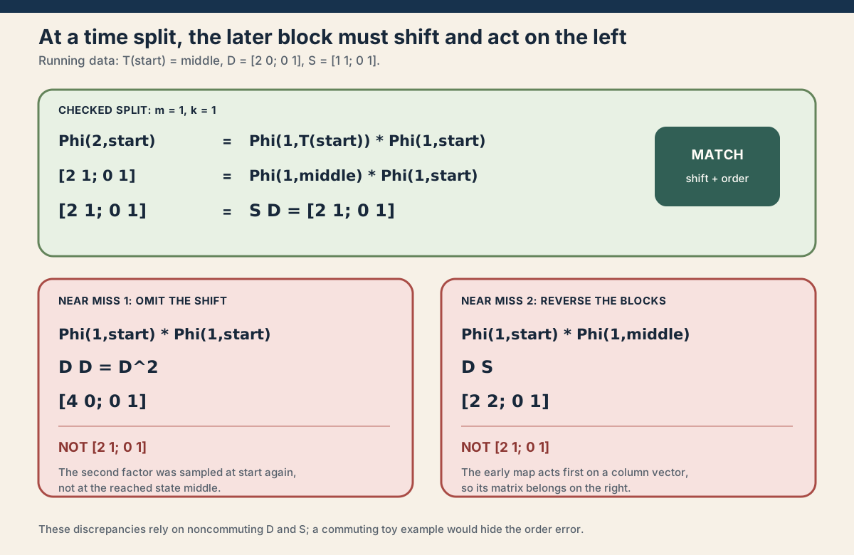
Return to the three-state example and split the two-step value after one step, so \(m=1\), \(k=1\), and \(\omega=\mathsf{start}\). The shift is
\[ T^1(\mathsf{start})=\mathsf{middle}. \]The right-hand side of the cocycle law is therefore
\[ \begin{aligned} \Phi(1,T(\mathsf{start}))\Phi(1,\mathsf{start}) &=\Phi(1,\mathsf{middle})\Phi(1,\mathsf{start})\\ &=SD\\ &= \begin{bmatrix}1&1\\0&1\end{bmatrix} \begin{bmatrix}2&0\\0&1\end{bmatrix}\\ &= \begin{bmatrix}2&1\\0&1\end{bmatrix}\\ &=\Phi(2,\mathsf{start}). \end{aligned} \]This is a numerical verification of the project convention, not its general proof. The Lean theorem proves the identity for every permitted semiring, finite matrix index type, base map, generator, two natural block lengths, and base point.
Near miss one: omit the shifted base point
If the later step starts at \(\mathsf{start}\) again, then it samples \(D\) twice:
\[ DD=D^2 {} = \begin{bmatrix}2&0\\0&1\end{bmatrix} \begin{bmatrix}2&0\\0&1\end{bmatrix} {} = \begin{bmatrix}4&0\\0&1\end{bmatrix}. \]That is not the true two-step value \(\left[\begin{smallmatrix}2&1\\0&1\end{smallmatrix}\right]\). The base shift is mathematical data, not bookkeeping decoration.
Near miss two: reverse the chronological blocks
If the early matrix is put on the left, the product becomes
\[ DS {} = \begin{bmatrix}2&0\\0&1\end{bmatrix} \begin{bmatrix}1&1\\0&1\end{bmatrix} {} = \begin{bmatrix}2&2\\0&1\end{bmatrix}. \]This also differs from the correct value. The example was chosen so \(D\) and \(S\) do not commute:
\[ SD= \begin{bmatrix}2&1\\0&1\end{bmatrix} \ne \begin{bmatrix}2&2\\0&1\end{bmatrix} =DS. \]A commuting example could accidentally hide an order error even though the general formula was wrong.
Camp five: complex measurability
Now equip \(\Omega\) with a measurable-space structure and specialize the matrix entries to \(\mathbb C\).
If \(T\) is measurable, then every natural iterate \(T^j\) is measurable. If the generator \(A\) is measurable, composition gives
\[ \omega\longmapsto A(T^j\omega) \]as a measurable matrix-valued map. The theorem
measurable_orbitMatrixSequence records this for every \(j\).
Its public type does not require finite matrix indices or decidable equality. No multiplication occurs in one orbit factor.
The theorem measurable_cocycleProduct then applies the preceding
finite-product measurability theorem. Every factor in the required prefix is
measurable because every orbit factor is measurable. The conclusion is
measurable for every finite \(k\).
This second theorem does require finite matrix indices and decidable equality because it multiplies matrices. Its complex scope matches the project’s checked measurable multiplication interface. The theorem does not form a pushforward law or prove integrability.
In Lean: measurable orbit factors are compositions
hA.comp (hT.iterate j)hTis a proof ofMeasurable T, not the mapTitself.hT.iterate jproves thatT^[j]is measurable.hAproves that the generatorAis measurable..compcomposes the two proofs in the same order as \(A\circ T^j\).- This expression is the proof body of
measurable_orbitMatrixSequence. It supplies ordinary measurability only: no measure, density, expectation, or integrability appears.
Camp six: what measure preserving means
Let \(\mu\) be a measure on \(\Omega\). Mathlib defines
MeasurePreserving T μ μ as a proposition with two fields:
Measurable T; andMeasure.map T μ = μ.
Mathematically,
\[ T_*\mu=\mu. \]For any measurable set \(B\), this yields
\[ \mu(T^{-1}(B))=\mu(B). \]The base transformation redistributes points without changing the measure of measurable events.
Preservation is not probability normalization
Nothing in MeasurePreserving T μ μ says
\(\mu(\Omega)=1\). The zero measure is preserved by every measurable self-map,
and infinite measures can also be invariant. A probability interpretation
needs a separate IsProbabilityMeasure μ assumption or a bundled
ProbabilityMeasure Ω. Neither appears in RMT-13.
Measure preservation can support a later proof that a measurable observable and its composition with a base iterate have the same raw pushforward measure. RMT-13 does not state that law-level theorem, and without probability normalization it does not package the orbit factors as identically distributed random variables. Invariance of one-factor marginals would still say nothing about independence between different times.
Preservation is not ergodicity
Ergodicity says, roughly, that invariant measurable events are trivial up to measure zero. Mixing asserts a stronger long-time loss of correlation. Measure preservation alone says neither. A base map can preserve many nontrivial invariant pieces.
Preservation is not invertibility
A noninjective map can preserve a measure. The structure stores an ordinary self-map, not an equivalence, so it supplies no backward orbit and no negative-time action.
Why one-sided time is a structural boundary
Natural-number time makes every forward expression meaningful without an inverse. The sequence
\[ \omega,\quad T\omega,\quad T^2\omega,\quad\ldots \]exists for every self-map. To define a value at time \(-1\), one would need to recover a previous environment and reverse a matrix update. That generally requires an invertible base and invertible generator values, together with a law relating the backward and forward definitions.
None of those data can be reconstructed from measure preservation alone. Even when a measure-preserving map is invertible almost everywhere, the present Lean field is an ordinary function with no stored measurable inverse. Likewise, a complex square matrix may be singular. The one-sided interface therefore avoids choosing a false inverse or hiding an exceptional set.
A future two-sided cocycle would naturally use integer time and an invertible measure-preserving base action. It would need an explicit inverse convention for negative matrix products. RMT-13 does not reserve such a convention by notation.
The namespace RandomCocycles by itself carries no assumption of a
complete metric dynamical system.
Camp seven: the bundled generator presentation
The central structure is:
structure DiscreteMatrixCocycle (μ : Measure Ω) where
  base : Ω → Ω
  generator : RandomMatrix Ω ι ι ℂ
  base_preserving : MeasurePreserving base μ μ
  measurable_generator : Measurable generator
The four fields have separate jobs:
| Field | What it stores | What it does not store |
|---|---|---|
base | One forward environment update | An inverse or group action |
generator | One complex matrix at each environment | A separately supplied time-indexed family |
base_preserving | Base measurability and invariance of \(\mu\) | Probability, ergodicity, or mixing |
measurable_generator | Ordinary measurability of the one-step matrix map | Integrability, independence, or a law |
The structure itself does not require Fintype ι or
DecidableEq ι. It can store a base and generator before asking for
finite matrix multiplication. Its value method does require those
finite-index assumptions because it forms products.
The bundle is generator presented. It does not store an independent \(\Phi\) field and a cocycle-law field. Instead,
\[ C.\operatorname{value}(k)= \operatorname{cocycleProduct}(C.\operatorname{base}, C.\operatorname{generator},k). \]The unbundled algebra then proves every value theorem.
In Lean: build a bundle from data and evidence
{ base := T, generator := A, base_preserving := hT, measurable_generator := hA }- Curly braces construct a structure value by naming its fields.
base := Tandgenerator := Astore the two functions.base_preserving := hTstores a proof ofMeasurePreserving T μ μ. That proof includes measurability ofTand equality of the pushforward withμ.measurable_generator := hAstores a proof ofMeasurable A.- There is no field for a probability normalization, inverse, ergodicity, independence, norm, limit, or Lyapunov exponent.
Camp eight: empty matrix dimension remains valid
The coordinate type \(\iota\) may be empty. It is still finite and has decidable equality. A square matrix on that type has no entries and exactly one value, which is the identity matrix.
Every orbit factor and cocycle value is therefore the unique matrix. The successor and addition laws remain true. Measurability is automatic, and the base measure-preservation statements are independent of matrix coordinates.
The theorem base_iterate_preserving explicitly omits finite-index
and decidable-equality assumptions because it concerns only the base map.
Likewise, measurable_orbitMatrixSequence needs neither assumption
because a single matrix-valued composition performs no multiplication.
No Nonempty ι assumption appears anywhere in the module. The
positive-dimension norm normalization from RMT-11 is irrelevant here because
RMT-13 defines no norm.
Camp nine: bundled values inherit every finite theorem
For a bundled cocycle \(C\), the project defines
C.value k by the unbundled cocycle product. It publishes:
The bundled addition law is
\[ C.\operatorname{value}(m+k,\omega) {} = C.\operatorname{value}(k,C.\operatorname{base}^m\omega) C.\operatorname{value}(m,\omega). \]The zero and successor equations are definitional. The one and addition theorems reuse their unbundled counterparts.
For measurability,
C.base_preserving.measurable extracts base measurability from the
preservation field. Combined with C.measurable_generator, it feeds
measurable_cocycleProduct. Thus
DiscreteMatrixCocycle.measurable_value proves ordinary
measurability for every finite value.
RMT-12 showed how a measurable random matrix can be pushed forward to a law.
RMT-13 does not perform that step. A later theorem may apply the earlier law
interface to C.value k, but no product-law declaration is exposed
here.
Camp ten: every natural base iterate preserves the measure
From
\[ T_*\mu=\mu, \]composition gives
\[ (T^k)_*\mu=\mu \]for every natural number \(k\). At \(k=0\), the identity map preserves \(\mu\). At a successor, the composition of two measure-preserving maps is measure preserving.
Mathlib packages this induction as
MeasurePreserving.iterate. The project theorem
DiscreteMatrixCocycle.base_iterate_preserving applies it directly:
theorem base_iterate_preserving
    (C : DiscreteMatrixCocycle (ι := ι) μ) (k : ℕ) :
    MeasurePreserving C.base^[k] μ μ :=
  C.base_preserving.iterate k
In Lean: every natural base iterate preserves the same measure
C.base_preserving.iterate kC.base_preservingselects the stored one-stepMeasurePreservingproof..iterate kapplies Mathlib’s finite-iteration theorem to that proof.- The result concerns
C.base^[k], the \(k\)-fold function iterate of the base. - The proof does not inspect
C.generatorand therefore needs no matrix-index assumptions. - Preservation of every finite iterate still does not make the base invertible, ergodic, or mixing.
This theorem says that each finite base shift retains the same measure. It does not say that an iterate is ergodic or mixing, and it does not prove invariance of a skew-product transformation that also updates vectors.
Type the running example yourself with Lean and Std
The project module uses Mathlib matrices, measurable spaces, measures, and
measure-preserving maps. You do not need that full dependency graph to check
the opening arithmetic. The worksheet below imports only Lean’s
Std library and models a \(2\)-by-\(2\) integer matrix as four
named entries.
This is a standalone tutorial. It is suitable for an ordinary macOS or Linux machine and does not invoke Lake or build Mathlib.
Save the exact block below as
/tmp/GeneratorCocycleTutorial.lean:
import Std

namespace GeneratorCocycleTutorial

inductive State where
  | start
  | middle
  | sink
  deriving Repr, DecidableEq

def base : State → State
  | .start => .middle
  | .middle => .sink
  | .sink => .sink

def baseIterate : Nat → State → State
  | 0, ω => ω
  | n + 1, ω => base (baseIterate n ω)

structure Matrix2 where
  a00 : Int
  a01 : Int
  a10 : Int
  a11 : Int
  deriving Repr, DecidableEq

def Matrix2.one : Matrix2 :=
  { a00 := 1, a01 := 0, a10 := 0, a11 := 1 }

def Matrix2.mul (A B : Matrix2) : Matrix2 :=
  { a00 := A.a00 * B.a00 + A.a01 * B.a10
    a01 := A.a00 * B.a01 + A.a01 * B.a11
    a10 := A.a10 * B.a00 + A.a11 * B.a10
    a11 := A.a10 * B.a01 + A.a11 * B.a11 }

instance : Mul Matrix2 where
  mul := Matrix2.mul

def Matrix2.entries (A : Matrix2) : List Int :=
  [A.a00, A.a01, A.a10, A.a11]

def generator : State → Matrix2
  | .start =>
      { a00 := 2, a01 := 0, a10 := 0, a11 := 1 }
  | .middle =>
      { a00 := 1, a01 := 1, a10 := 0, a11 := 1 }
  | .sink =>
      { a00 := 1, a01 := 0, a10 := 1, a11 := 1 }

def cocycle : Nat → State → Matrix2
  | 0, _ => Matrix2.one
  | n + 1, ω =>
      generator (baseIterate n ω) * cocycle n ω

def splitAtOne (ω : State) : Matrix2 :=
  cocycle 1 (baseIterate 1 ω) * cocycle 1 ω

def omitShiftAtTwo (ω : State) : Matrix2 :=
  generator ω * generator ω

def reverseOrderAtTwo (ω : State) : Matrix2 :=
  generator ω * generator (base ω)

#eval [(cocycle 0 .start).entries,
  (cocycle 1 .start).entries,
  (cocycle 2 .start).entries]

#eval [(cocycle 0 .middle).entries,
  (cocycle 1 .middle).entries,
  (cocycle 2 .middle).entries]

#eval [(cocycle 2 .start).entries,
  (splitAtOne .start).entries]

#eval decide (cocycle 2 .start = splitAtOne .start)

#eval [(omitShiftAtTwo .start).entries,
  (reverseOrderAtTwo .start).entries]

#eval [decide (cocycle 2 .start ≠ omitShiftAtTwo .start),
  decide (cocycle 2 .start ≠ reverseOrderAtTwo .start)]

example : base .middle = base .sink := by decide
example : State.middle ≠ State.sink := by decide
example : cocycle 0 .start = Matrix2.one := by decide
example : cocycle 1 .start = generator .start := by decide
example : cocycle 2 .start =
    cocycle 1 (baseIterate 1 .start) * cocycle 1 .start := by decide
example : cocycle 2 .start ≠ omitShiftAtTwo .start := by decide
example : cocycle 2 .start ≠ reverseOrderAtTwo .start := by decide

end GeneratorCocycleTutorial
Open a terminal and type:
source "$HOME/.elan/env"
elan run leanprover/lean4:v4.32.0 lean \
  /tmp/GeneratorCocycleTutorial.lean
The pinned version in the command matters: it makes the tutorial replay the
same Lean release as formalization/lean-toolchain. This exact
worksheet was executed successfully with Lean 4.32.0 while editing the
chapter. Its output was:
[[1, 0, 0, 1], [2, 0, 0, 1], [2, 1, 0, 1]]
[[1, 0, 0, 1], [1, 1, 0, 1], [1, 1, 1, 2]]
[[2, 1, 0, 1], [2, 1, 0, 1]]
true
[[4, 0, 0, 1], [2, 2, 0, 1]]
[true, true]
Each four-number list is a matrix in row order:
[a00, a01, a10, a11].
- The first line is the start ledger \(I,D,SD\).
- The second is the shifted middle ledger \(I,S,LS\).
- The third prints the direct two-step value and the one-plus-one split; the lists agree.
- The standalone
trueis the result of deciding that equality. - The fifth line prints the omitted-shift value \(D^2\) and the reversed value \(DS\).
- The last line reports
truefor both comparisons with \(SD\).
The example commands contain kernel-checked propositions. The
first two show the base is noninjective: middle and sink are different inputs
with the same image. The remaining example declarations record the stated
zero value, one-step value, numeric cocycle split, and two inequalities for
this finite model; their proof terms are kernel checked.
The worksheet mirrors the project’s recursion but is not a substitute for the project theorem. It uses integer entries, a hand-written matrix multiplication, one three-state example, and concrete decidable propositions. It does not formalize arbitrary semirings, Mathlib matrices, measurability, measure preservation, empty matrix dimension, or the general cocycle identity.
The complete declaration map
The module exposes exactly sixteen public declarations.
| Declaration | Layer | Exact role |
|---|---|---|
orbitMatrixSequence | Pure function layer | Evaluates one generator along every natural base iterate |
cocycleProduct | Semiring algebra | Forms the newest-factor-left product of the orbit sequence |
cocycleProduct_zero | Semiring algebra | The zero-horizon product is the constant identity map |
cocycleProduct_succ | Semiring algebra | Samples the generator at the newest base iterate and multiplies it on the left |
cocycleProduct_one | Semiring algebra | The one-step product is the generator |
cocycleProduct_add | Semiring algebra | Splits a product into a shifted later block on the left and an early block on the right |
measurable_orbitMatrixSequence | Complex measurability | Measurable base and generator give a measurable factor at every iterate |
measurable_cocycleProduct | Complex measurability | Every finite cocycle product is measurable |
DiscreteMatrixCocycle | Bundled presentation | Stores a base, complex generator, base-preservation proof, and generator-measurability proof |
DiscreteMatrixCocycle.value | Bundled finite value | Builds the cocycle product from the stored base and generator |
DiscreteMatrixCocycle.value_zero | Bundled algebra | The zero value is the identity map |
DiscreteMatrixCocycle.value_one | Bundled algebra | The one-step value is the stored generator |
DiscreteMatrixCocycle.value_succ | Bundled algebra | The newest sampled generator factor is multiplied on the left |
DiscreteMatrixCocycle.value_add | Bundled algebra | The bundled value satisfies the pointwise one-sided cocycle law |
DiscreteMatrixCocycle.measurable_value | Bundled measurability | Every finite bundled value is ordinarily measurable |
DiscreteMatrixCocycle.base_iterate_preserving | Base dynamics | Every natural iterate of the stored base preserves \(\mu\) |
The exact assumption ledger is:
| Interface | Assumptions |
|---|---|
orbitMatrixSequence | No scalar algebra, finite-index, measurable-space, or measure assumptions |
| Unbundled product algebra | Finite index type, decidable equality, scalar semiring |
| One orbit-factor measurability | Measurable space on \(\Omega\), complex matrices, measurable base and generator; no finite-index assumptions |
| Product measurability | The preceding measurable data plus finite index type and decidable equality |
DiscreteMatrixCocycle μ storage | Measurable space on \(\Omega\); no finite-index assumptions and no probability normalization |
| Bundled values and value algebra | Stored cocycle plus finite index type and decidable equality |
| Bundled value measurability | Stored preservation and generator evidence plus finite index type and decidable equality |
| Base-iterate preservation | Stored cocycle only; matrix finiteness and decidable equality are omitted |
No declaration assumes a nonempty coordinate type.
Proof architecture
The implementation is small because it composes established layers:
| Goal | Main ingredients |
|---|---|
| Orbit sequence | Function.iterate and function evaluation |
| Cocycle product | RMT-12 sampleForwardProduct |
| Zero and successor products | Definitional reduction |
| One-step product | Function extensionality, zeroth iterate, one-step product |
| Cocycle addition law | Induction on later length, iterate addition, product recursion, associativity |
| Orbit-factor measurability | Measurable.iterate and measurable composition |
| Product measurability | RMT-12 exact-prefix theorem applied to every orbit factor |
| Bundled values | Reuse the unbundled definitions and theorems |
| Bundled value measurability | Extract base measurability from measure preservation |
| Base-iterate preservation | Mathlib’s MeasurePreserving.iterate |
The central design choice is vertical reuse:
\[ \text{function iteration} \longrightarrow \text{orbit factors} \longrightarrow \text{measurable finite products} \longrightarrow \text{generator-presented cocycle}. \]No parallel matrix-product abstraction is introduced.
Why this layer matters for mathematics and physics
Random linear systems
A random linear recurrence can be written
\[ x_{k+1}(\omega) {} = A(T^k\omega)x_k(\omega). \]Its finite solution is
\[ x_k(\omega)=\Phi(k,\omega)x_0. \]The cocycle identity then expresses consistency across a time split: evolve for \(m\) steps, shift the environment, then evolve for \(k\) more.
RMT-13 defines the matrix value but no state-vector recurrence theorem. That action bridge can be added later from existing matrix-vector multiplication.
Transfer matrices
In finite disordered chains, a base state can encode the disorder environment and the generator can select the local transfer matrix. Moving the base exposes the next local environment. The product composes finite transfer steps.
This interpretation needs model-specific choices of \(\Omega\), \(T\), \(A\), and \(\mu\). Independence, stationarity in a probabilistic sense, and physical observables are not automatic.
Tangent dynamics
For a differentiable nonlinear map \(f\), the derivative matrices along an orbit formally resemble
\[ A(x)=Df(x), \qquad T(x)=f(x). \]The chain rule then turns derivatives of iterates into an ordered matrix product. RMT-13 does not define differentiability, derivatives, invariant domains, or that chain-rule bridge. The resemblance identifies a future consumer of the interface, not a theorem already proved.
Multiplicative ergodic theory
Lyapunov exponents study asymptotic logarithmic growth, often through
\[ \lim_{k\to\infty} \frac{1}{k}\log\lVert\Phi(k,\omega)\rVert. \]This expression requires a chosen matrix norm, measurability of the norm observable, policies for zero norm, logarithmic integrability, suitable invariant probability structure, and an asymptotic theorem. Invariant splittings need still more.
RMT-13 supplies only the finite measurable cocycle and preservation of the base measure. It does not establish any condition in that later analytic ledger except finite-value measurability.
Keep four interfaces on separate shelves
| Interface | Data or conclusion | Status here |
|---|---|---|
| Deterministic generator presentation | A point \(\omega\), a forward map \(T\), one generator \(A\), and each finite product \(\Phi(k,\omega)\) | The algebraic core is defined and checked |
| Random law | A measure on \(\Omega\), pushforward distributions of \(A\) or \(\Phi(k,\cdot)\), and possibly dependence assumptions | A measure is stored only in the bundle’s preservation field; no matrix law or independence theorem is defined |
| Invertible two-sided cocycle | Integer time, a backward base action, invertible factors, and a consistent negative-time product | Not defined; time is \(\mathbb N\) and the base need not be injective |
| Norm-growth limit or Lyapunov theory | A matrix norm, logarithmic observable, integrability, a limit theorem, and perhaps an invariant splitting | Not defined or proved in this module |
A finite value such as \(\Phi(2,\mathsf{start})=\left[\begin{smallmatrix}2&1\\0&1\end{smallmatrix}\right]\) is not a norm-growth limit. Even proving convergence of one scalar quantity \(k^{-1}\log\lVert\Phi(k,\omega)\rVert\) would not by itself construct the full collection of Lyapunov exponents or an Oseledets splitting. Those are different theorem layers with different hypotheses.
Common wrong turns
Treating the generator as an arbitrary time sequence
There is one map \(A:\Omega\to M_\iota(\mathbb C)\). Time dependence arises by evaluating it at \(T^j\omega\). An arbitrary family \(A_j(\omega)\) belongs to the preceding finite-random-product layer and need not be a cocycle generator.
Forgetting the shifted environment
The later block begins at \(T^m\omega\). Writing \(\Phi(k,\omega)\Phi(m,\omega)\) generally repeats factors from the beginning of the orbit.
Putting the early block on the left
The early block acts first on column vectors and is written on the right. The later block acts second and is written on the left.
Reading Function.iterate as matrix power
T^[j] iterates the base function. Matrix powers use a different
operation. The generator is evaluated after function iteration and only then
are matrices multiplied.
Assuming the bundle stores a cocycle-law axiom
The structure stores base data, generator data, and two evidence fields. Its value and cocycle law are derived from the generator presentation.
Equating measure preservation with probability
The source \(\mu\) is an arbitrary measure. Total mass one is not a field or theorem of this module.
Equating measure preservation with ergodicity or mixing
An invariant measure can support nontrivial invariant subsets and persistent correlations. Those stronger properties need separate definitions.
Assuming one-sided time can run backward
Natural-number iteration supplies no negative indices. The base and generator matrices need not be invertible.
Inferring a product-law factorization
The module defines no law of C.value k. Even after forming one,
matrix-factor dependence prevents a factorization without additional
hypotheses.
Reading finite measurability as integrability
A measurable norm or log norm can fail to be integrable. RMT-13 defines neither observable.
Reading the cocycle law as a Lyapunov theorem
The cocycle law is finite algebra. It creates no asymptotic limit, exponent, invariant splitting, or stability classification.
Assuming a nonlinear Jacobian bridge
The module contains no nonlinear map, derivative, chain rule, or theorem identifying the generator with a Jacobian matrix.
Exercises from trailhead to summit
Trailhead
- Write the base states and generator factors through time four.
- Expand \(\Phi(k,\omega)\) for \(k=0,1,2,3,4\).
- Explain why \(A(T^0\omega)=A(\omega)\).
- Show that
orbitMatrixSequenceneeds no semiring. - Verify the three-state horizon-zero, one, and two ledgers by hand.
Mid-mountain
- Split a five-step product after \(m=2\) and write every shifted factor.
- Prove the cocycle identity directly by expanding both sides.
- Reproduce the induction on \(k\), naming the iterate-addition and associativity steps.
- Construct a measure-preserving base that is not ergodic.
- Explain why the identity base preserves every measure but is usually not mixing.
- Prove measurability of one orbit factor by composing the generator with a base iterate.
- Explain why product measurability needs finite matrix indices while orbit-factor measurability does not.
Summit
- Compare the generator-presented structure with an abstract structure that stores \(\Phi\), normalization, and the cocycle law as fields.
- Prove on paper that every natural iterate of a measure-preserving map preserves the measure.
- Analyze the empty-coordinate-type cocycle and identify the unique matrix at every horizon.
- Define a candidate skew-product map on environments and column vectors. List the additional measure on vector space and invariance theorem that RMT-13 does not provide.
- Define a finite norm observable on paper. List norm choice, measurability, zero-norm, and integrability decisions needed before using its logarithm.
- State the probability, invariance, and logarithmic-integrability hypotheses a future multiplicative ergodic theorem would need.
- Formulate a derivative-product theorem for iterates of a differentiable map and list the chain-rule hypotheses absent here.
Inspect and check the exact project interfaces
The authoritative source is
formalization/NonlinearDynamics/Random/RandomCocycles/Discrete.lean.
For a full project check, install the repository’s pinned dependencies and
put the following lines in a temporary project scratch file:
import NonlinearDynamics.Random.RandomCocycles.Discrete

open Matrix MeasureTheory
open NonlinearDynamics.Random.RandomCocycles

#check orbitMatrixSequence
#check cocycleProduct
#check cocycleProduct_zero
#check cocycleProduct_succ
#check cocycleProduct_one
#check cocycleProduct_add
#check measurable_orbitMatrixSequence
#check measurable_cocycleProduct
#print DiscreteMatrixCocycle
#check DiscreteMatrixCocycle.value
#check DiscreteMatrixCocycle.value_zero
#check DiscreteMatrixCocycle.value_one
#check DiscreteMatrixCocycle.value_succ
#check DiscreteMatrixCocycle.value_add
#check DiscreteMatrixCocycle.measurable_value
#check DiscreteMatrixCocycle.base_iterate_preserving
import loads this project module and its pinned Mathlib
dependencies. #check elaborates an existing
declaration and reports its type. #print exposes the four structure
fields. These commands do not sample matrices, infer a probability law, or
prove a Lyapunov theorem.
From the repository root, the exact per-file command is:
cd formalization
lake env lean NonlinearDynamics/Random/RandomCocycles/Discrete.lean
This full project check may compile substantial dependencies and therefore may require substantial disk space and memory.
cd formalization
lake env lean -DwarningAsError=true NonlinearDynamics/Random/RandomCocycles/Discrete.lean
Resource note: this exact file uses the repository's
pinned Lean and Mathlib dependencies. Initial project setup can require
substantial disk space and build time. For a lightweight first step on
macOS or Linux, use the page's standalone Lean-core or Std
tutorial.
Passing a technical check still does not complete human or Pro review.
Summit: what has and has not been proved
| Topic | Status in this module |
|---|---|
| Generator sampled along every natural base iterate | Defined |
| Newest-factor-left finite cocycle product | Defined over every scalar semiring |
| Zero, one, and successor values | Checked |
| Later-block-left pointwise one-sided cocycle identity | Checked |
| Measurability of every complex orbit factor | Checked |
| Measurability of every finite complex cocycle value | Checked |
| Generator-presented bundle over a measure-preserving base | Defined |
| Ordinary measurability of the bundled generator | Stored |
| Ordinary measurability of every bundled finite value | Checked |
| Preservation of \(\mu\) by every natural base iterate | Checked |
| Empty matrix coordinate type | Supported |
| Probability normalization of \(\mu\) | Not assumed or proved |
| Pushforward law of a cocycle value | Not defined |
| Ergodicity or mixing | Not assumed or proved |
| Independent-and-identically-distributed factor model | Not assumed or proved |
| Invertibility of base, factors, or cocycle values | Not assumed |
| Negative-time extension | Not defined |
| Two-sided group cocycle | Not defined |
| Skew-product invariance | Not stated |
| Product-law factorization | Not stated |
| Matrix norm or norm observable | Not chosen or defined |
| Norm or logarithmic-norm integrability | Not proved |
| Lyapunov exponent or asymptotic growth limit | Not defined or proved |
| Oseledets theorem or invariant splitting | Not invoked |
| Derivative or Jacobian product along a nonlinear orbit | Not connected |
| Stability, bifurcation, chaos, or physical-model theorem | Not claimed |
The new summit is structural: one measurable generator over a measure-preserving forward base now produces a checked finite matrix cocycle. Nothing in that sentence silently grants probability, ergodicity, analytic growth, or asymptotic theory.
Where to continue
Finite-Time Norm and Extended-Log-Norm Observables for Matrix Cocycles is the immediate successor. It keeps this chapter’s finite, one-sided cocycle and adds a measurable maximum-row-sum norm observable, a zero-aware extended log norm, and subadditivity across the shifted split. The extended log-norm observable entry is the compact guide to the new endpoint and dimension policy.
The one-sided discrete matrix cocycle glossary entry is the compact guide to the base orbit, generator presentation, and shifted split law.
Measurable Finite Random-Matrix Products and Proof-Carrying Pushforward Laws develops the immediate product and measurability layer below this cocycle. Ordered Finite Matrix Products and Operator-Norm Growth develops the deterministic chronology and a specific finite norm bound.
RMT-14 now defines the finite norm and extended-log-norm observables without claiming asymptotic exponents. Integrability, normalized growth, and the hypotheses of subadditive or multiplicative ergodic theorems remain later layers.
References
Mathlib contributors.
Function iteration,
Mathlib 4 documentation. This official source defines natural-number
Function.iterate and its zero, successor, and addition laws.
Mathlib contributors. Measure-preserving maps, Mathlib 4 documentation. This official source defines measure preservation as measurability plus pushforward equality and proves preservation under composition and natural-number iteration.
Ludwig Arnold. Random Dynamical Systems, Springer Monographs in Mathematics, 1998. This develops cocycles over metric dynamical systems and the multiplicative ergodic setting. Its usual probability, base-flow, integrability, and asymptotic hypotheses are future layers here.
V. I. Oseledets. A multiplicative ergodic theorem. Characteristic Ljapunov exponents of dynamical systems, Transactions of the Moscow Mathematical Society 19 (1968), 197-231. This primary source supplies the historical theorem behind Lyapunov exponents and invariant splittings. RMT-13 establishes none of its analytic or asymptotic hypotheses or conclusions.
The exact upstream Lean source audited for this chapter is Mathlib commit
81a5d257,
the revision pinned by formalization/lake-manifest.json.