Start with one exact two-by-two perturbation
Let
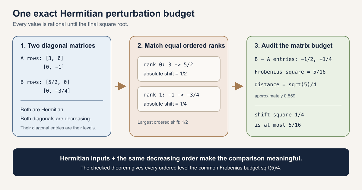
\[ A= \begin{bmatrix} 3&0\\ 0&-1 \end{bmatrix}, \qquad B= \begin{bmatrix} \frac52&0\\ 0&-\frac34 \end{bmatrix}. \]Both matrices are Hermitian : each equals its conjugate transpose. Because the diagonal entries are already decreasing, their ordered eigenvalue vectors are visible without a characteristic-polynomial calculation:
An eigenvalue \(\lambda\) of a matrix \(M\) is a scalar for which \(Mv=\lambda v\) for some nonzero vector \(v\). For a diagonal matrix, the diagonal entries are its eigenvalues, including multiplicity.
\[ \Lambda(A)=(3,-1), \qquad \Lambda(B)=\left(\frac52,-\frac34\right). \]Match equal positions in these decreasing lists. The two level shifts are
\[ \left|3-\frac52\right|=\frac12, \qquad \left|-1-\left(-\frac34\right)\right|=\frac14. \]The matrix difference is
\[ A-B= \begin{bmatrix} \frac12&0\\ 0&-\frac14 \end{bmatrix}. \]Its squared Frobenius norm is the sum of the squared entry magnitudes:
\[ \lVert A-B\rVert_F^2 =\left(\frac12\right)^2+\left(-\frac14\right)^2 =\frac14+\frac1{16} =\frac5{16}. \]Therefore
\[ \lVert A-B\rVert_F=\frac{\sqrt5}{4}\approx0.559. \]The larger ordered shift is \(1/2=0.5\), so both coordinates satisfy
\[ \left|\lambda_i(A)-\lambda_i(B)\right| \le \frac12 \le \frac{\sqrt5}{4} =\lVert A-B\rVert_F. \]Nothing statistical happened. We selected two deterministic matrices, computed their deterministic spectra, and checked one deterministic inequality. Squaring is legitimate in the exact ledger because every compared quantity is nonnegative:
\[ \left(\frac12\right)^2=\frac4{16}\le\frac5{16}. \]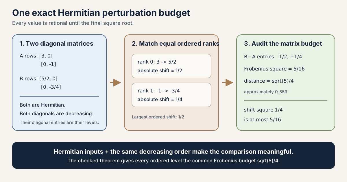
Two near-misses show why the hypotheses matter
Near-miss A: reverse one eigenvalue list
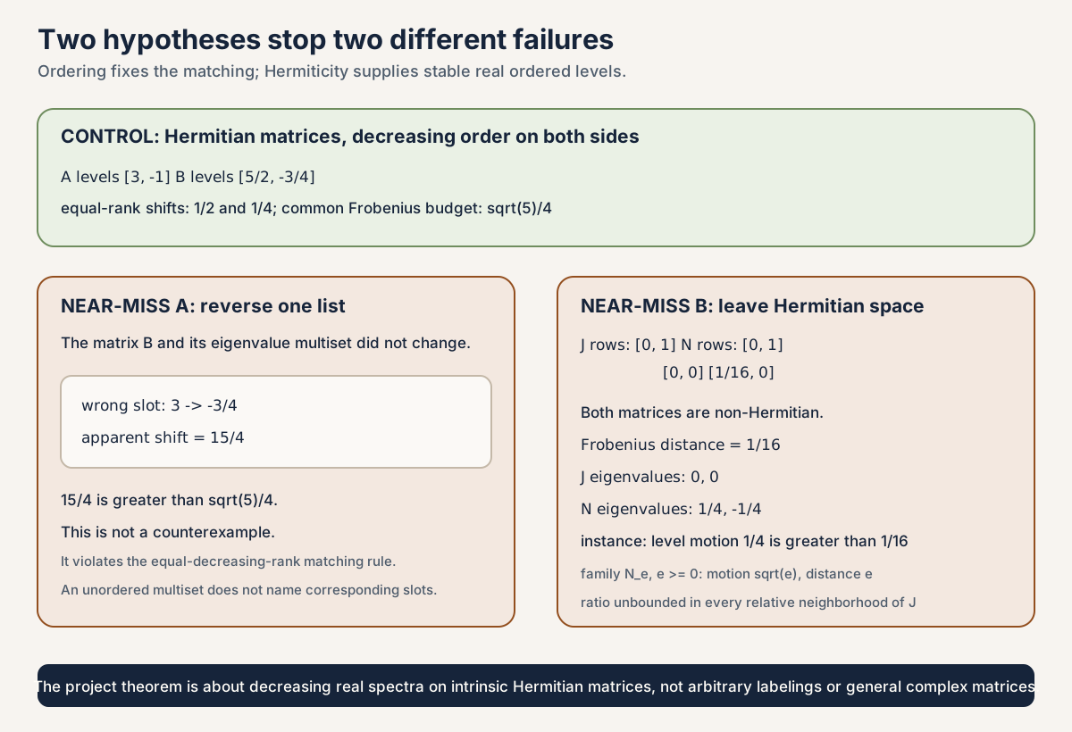
Keep the same matrix \(B\), but write its eigenvalues in the opposite order:
\[ \left(-\frac34,\frac52\right). \]Comparing the first slot of that list with the first slot of \(\Lambda(A)\) produces
\[ \left|3-\left(-\frac34\right)\right| =\frac{15}{4} \gt\frac{\sqrt5}{4}. \]This is not a counterexample. The theorem compares equal positions after both Hermitian spectra have been sorted in the same decreasing order. An unordered multiset records which eigenvalues exist, but it does not by itself say which one on the left corresponds to which one on the right.
Near-miss B: leave the Hermitian world
Now consider two real, but non-Hermitian, matrices:
\[ J= \begin{bmatrix} 0&1\\ 0&0 \end{bmatrix}, \qquad N= \begin{bmatrix} 0&1\\ \frac1{16}&0 \end{bmatrix}. \]Their Frobenius distance is only
\[ \lVert J-N\rVert_F=\frac1{16}. \]Both matrices are non-Hermitian, even though the eigenvalues in this exact pair happen to be real.
The characteristic polynomial is \(\det(tI-M)\); its roots are the eigenvalues. The characteristic polynomial of \(J\) is \(t^2\), so both eigenvalues are zero. The characteristic polynomial of \(N\) is \(t^2-\frac1{16}\), so its eigenvalues are \(1/4\) and \(-1/4\). Thus one level moves by
\[ \frac14\gt\frac1{16}. \]The single pair is a counterexample to extending the Hermitian theorem’s constant \(1\) to all real \(2\)-by-\(2\) matrices that happen to have real spectra when those real eigenvalues are matched in decreasing order. It says nothing about every possible non-Hermitian spectral metric or matching convention. To see the stronger local failure along this particular real-spectrum family, use
\[ N_\varepsilon= \begin{bmatrix} 0&1\\ \varepsilon&0 \end{bmatrix}, \qquad \varepsilon\gt0. \]Then \(J=N_0\), \(\lVert N_\varepsilon-J\rVert_F=\varepsilon\), and the roots of \(t^2-\varepsilon\) are \(\pm\sqrt{\varepsilon}\). The ratio of eigenvalue motion to matrix motion is
\[ \frac{\sqrt{\varepsilon}}{\varepsilon} =\frac1{\sqrt{\varepsilon}} \longrightarrow\infty \qquad\text{as }\varepsilon\downarrow0. \]Thus, along the one-sided family \(\{N_\varepsilon:\varepsilon\ge0\}\), no fixed finite Lipschitz constant works in any relative neighborhood of the defective matrix \(J\) for the decreasingly ordered real-eigenvalue map. This is a family-specific local statement, not a global theorem about every way to compare complex spectra. The matrix \(J\) is defective because it does not have enough linearly independent eigenvectors to form a basis. Hermiticity supplies the stable min-max geometry used by the project proof. The checked theorem makes no non-Hermitian perturbation claim.
Type the exact finite ledger with Lean and Std
The general eigenvalue theorem is a full project check: it imports Mathlib
and may require substantial disk space and memory. Its decisive rational
arithmetic fits in a standalone tutorial importing only Lean’s
Std library. This
tutorial represents the two diagonal spectra directly and checks the
non-Hermitian eigenvalues by evaluating their characteristic polynomials. It
does not formalize matrix spectral theory.
Save the following exact file as
/tmp/HermitianPerturbation2.lean on a normal Mac or Linux host:
import Std

namespace HermitianPerturbation2

def sq (x : Rat) : Rat := x * x

def absRat (x : Rat) : Rat :=
  if x < 0 then -x else x

def aSpectrum : List Rat := [3, -1]

def bSpectrum : List Rat := [(5 : Rat) / 2, (-3 : Rat) / 4]

def orderedShifts : List Rat :=
  [absRat (3 - (5 : Rat) / 2), absRat (-1 - (-3 : Rat) / 4)]

def frobeniusSq : Rat :=
  sq (3 - (5 : Rat) / 2) + sq (-1 - (-3 : Rat) / 4)

def maxOrderedShift : Rat :=
  max (absRat (3 - (5 : Rat) / 2)) (absRat (-1 - (-3 : Rat) / 4))

def reversedSlotShift : Rat :=
  absRat (3 - (-3 : Rat) / 4)

structure Matrix2 where
  a11 : Rat
  a12 : Rat
  a21 : Rat
  a22 : Rat
deriving Repr, DecidableEq

def trace (M : Matrix2) : Rat := M.a11 + M.a22

def det (M : Matrix2) : Rat := M.a11 * M.a22 - M.a12 * M.a21

def charAt (M : Matrix2) (lambda : Rat) : Rat :=
  sq lambda - trace M * lambda + det M

def frobeniusSqDiff (M N : Matrix2) : Rat :=
  sq (M.a11 - N.a11) + sq (M.a12 - N.a12) +
    sq (M.a21 - N.a21) + sq (M.a22 - N.a22)

def jordan : Matrix2 :=
  { a11 := 0, a12 := 1, a21 := 0, a22 := 0 }

def perturbedJordan : Matrix2 :=
  { a11 := 0, a12 := 1, a21 := (1 : Rat) / 16, a22 := 0 }

#eval orderedShifts
#eval frobeniusSq
#eval (sq maxOrderedShift, decide (sq maxOrderedShift <= frobeniusSq))
#eval (reversedSlotShift, decide (sq reversedSlotShift <= frobeniusSq))
#eval [charAt jordan 0, charAt perturbedJordan ((1 : Rat) / 4),
  charAt perturbedJordan ((-1 : Rat) / 4)]
#eval (frobeniusSqDiff jordan perturbedJordan, sq ((1 : Rat) / 4),
  decide (sq ((1 : Rat) / 4) <= frobeniusSqDiff jordan perturbedJordan))

example : orderedShifts = [(1 : Rat) / 2, (1 : Rat) / 4] := by
  native_decide
example : frobeniusSq = (5 : Rat) / 16 := by native_decide
example : sq maxOrderedShift <= frobeniusSq := by native_decide
example : not (sq reversedSlotShift <= frobeniusSq) := by native_decide
example : charAt jordan 0 = 0 := by native_decide
example : charAt perturbedJordan ((1 : Rat) / 4) = 0 := by native_decide
example : charAt perturbedJordan ((-1 : Rat) / 4) = 0 := by native_decide
example : frobeniusSqDiff jordan perturbedJordan = (1 : Rat) / 256 := by
  native_decide
example : not (sq ((1 : Rat) / 4) <=
    frobeniusSqDiff jordan perturbedJordan) := by native_decide

end HermitianPerturbation2
Type:
source "$HOME/.elan/env"
elan run leanprover/lean4:v4.32.0 lean \
  /tmp/HermitianPerturbation2.lean
The exact worksheet was executed successfully with Lean 4.32.0. It printed:
[(1 : Rat)/2, (1 : Rat)/4]
(5 : Rat)/16
((1 : Rat)/4, true)
((15 : Rat)/4, false)
[0, 0, 0]
((1 : Rat)/256, (1 : Rat)/16, false)
The first Boolean records the squared Hermitian budget. The second rejects the
reversed-slot comparison. The three zeros are exact evaluations showing that
\(0\) is a root for \(J\) and that \(1/4,-1/4\) are roots for \(N\). The last
tuple compares the squared non-Hermitian matrix distance \(1/256\) with the
squared level motion \(1/16\) and correctly returns false.
Rat provides exact rational arithmetic. decide
computes a boolean decision for a proposition, while
native_decide closes a proposition by trusted kernel-checked
reflection after native evaluation. The worksheet checks the finite ledger,
not the general eigenvalue theorem, continuity, measurability, or any
probability law.
What the checked module proves
The preceding spectral layer attached a decreasing real eigenvalue vector to every finite intrinsic Hermitian matrix. It then turned that vector into a spectral counting measure and a zero-aware empirical spectral measure . Those constructions were algebraically complete, but their measure-valued maps were conditionally measurable: each theorem asked the caller to prove that every ordered eigenvalue coordinate was measurable.
RMT-10B closes that seam. Its central deterministic estimate is
\[ \boxed{ \left|\lambda_i(A)-\lambda_i(B)\right| \le \lVert A-B\rVert_F } \]for two \(n\)-by-\(n\) Hermitian matrices \(A\) and \(B\), with both spectra listed in decreasing order and \(i\in\operatorname{Fin}(n)\). The norm is the intrinsic Hermitian Frobenius norm .
The estimate is strong enough to make each coordinate 1-Lipschitz and the full ordered vector 1-Lipschitz for the finite function-space sup metric. Lipschitz maps are continuous; continuous maps between the Borel spaces in use are measurable. Here a Borel measurable structure is generated by the open sets of the surrounding topology. The conditional measure-valued interfaces from RMT-10A can therefore be discharged, including the equality between the empirical-spectral pushforwards of the ambient and intrinsic Gaussian unitary ensemble (GUE) laws.
The proof is deliberately finite and structural. It does not import an operator-norm Weyl theorem. Instead it builds an ordered eigenbasis, forms top and bottom spectral subspaces, forces them to intersect by dimension, and uses a vector in that intersection to compare two quadratic forms. That route makes every hypothesis and every norm visible in Lean.
Three layers that must not collapse
The word “spectrum” can refer to several typed objects here. Keep this ledger
in view. Write \(\mathcal H_n\) for the space of \(n\)-by-\(n\) Hermitian
matrices with the intrinsic Frobenius metric. Mathlib’s Giry measurable
structure on Measure ℝ is generated by the evaluation maps
\(\mu\mapsto\mu(S)\) for measurable sets \(S\). It lets a measure itself be the
output of a measurable map without first choosing a topology on the space of
measures.
| Layer | Exact object | What RMT-10B proves | What it does not yet do |
|---|---|---|---|
| Deterministic ordered spectrum | \(\Lambda:\mathcal H_n\to(\operatorname{Fin}(n)\to\mathbb R)\) | Frobenius 1-Lipschitz, continuous, and Borel measurable | Select a random matrix or define a probability law |
| Deterministic measure-valued observable | \(L:\mathcal H_n\to\operatorname{Measure}(\mathbb R)\) | Giry measurability of counting and empirical spectral maps | Prove weak or Wasserstein continuity, or produce a density |
| Random output law | \(\mu\mapsto L_*\mu\) after a source law \(\mu\) is supplied | Equality of the ambient and intrinsic GUE pushforwards already present in the API | Introduce the later dedicated name, calculate its density, or prove an asymptotic law |
A measurable function is a deterministic map with a preimage property. A pushforward uses such a map together with an input measure to create an output measure. A probability law is therefore not another word for continuity or measurability. RMT-10B proves the map properties first and invokes the existing GUE input laws only in its final theorem.
Choose a route up
| Route | Begin with | Destination |
|---|---|---|
| First encounter | The exact two-by-two perturbation | Compute the ordered shifts and Frobenius budget before meeting the general theorem |
| Hands-on route | The standalone worksheet | Check the rational ledger locally without Mathlib or Lake |
| Norm route | Frobenius control of matrix-vector multiplication | Prove the analytic estimate that bounds quadratic-form change |
| Spectral route | Reindex the eigenbasis in the same order | Align eigenvectors with the decreasing eigenvalue API |
| Min-max route | Top and bottom spectral subspaces | Build the nonzero intersection witness |
| Inequality route | The one-sided Weyl estimate | Derive the absolute coordinate bound |
| Topology route | From coordinates to a Lipschitz vector | Separate coordinate and finite sup-metric claims |
| Probability route | From continuity to Giry measurability | Remove the earlier measure-valued hypotheses |
| Physics route | Energy levels under a Hamiltonian perturbation | Interpret the theorem without inventing a probabilistic result |
| Lean audit route | The complete public API | Map every public declaration to its exact role |
Learning objectives
By the summit, you should be able to:
- distinguish the Frobenius norm from the spectral operator norm;
- derive the matrix-vector estimate used by the proof;
- explain why the eigenbasis must be reindexed by the same order-preserving cast as the eigenvalue vector;
- expand a Hermitian quadratic form as a weighted sum of squared eigenbasis coordinates;
- define the top \(i+1\) and bottom \(n-i\) spectral subspaces;
- prove that those two subspaces have a nonzero intersection;
- explain why the intersection vector is the finite min-max witness;
- derive the one-sided ordered-eigenvalue estimate;
- obtain the absolute bound by swapping the two matrices;
- state the coordinatewise 1-Lipschitz theorem;
- identify the whole-vector target metric as the finite sup metric rather than an \(\ell^2\) eigenvalue metric;
- follow the implication from Lipschitz to continuous to measurable;
- explain how coordinate measurability makes a finite Dirac sum measurable;
- state the now-unconditional counting, empirical, and ambient spectral measurability theorems;
- draw the intrinsic-versus-ambient GUE pushforward square;
- distinguish eigenvalue continuity from eigenvector continuity;
- distinguish this theorem from Hoffman-Wielandt and Davis-Kahan; and
- list the density, concentration, differentiability, gap, and asymptotic results that RMT-10B does not prove.
The result in one picture
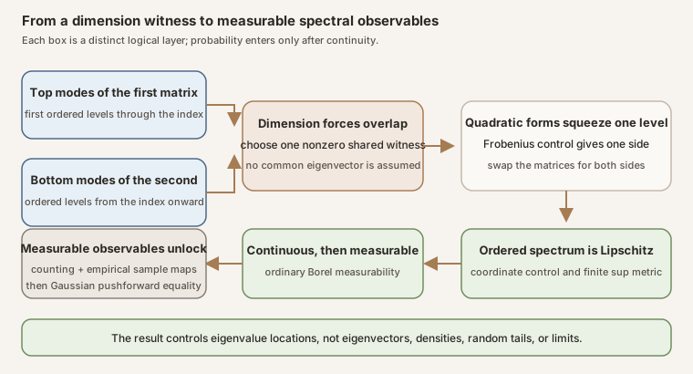
The figure compresses three mathematical layers that must stay separate:
- Linear algebra: an ordered eigenbasis and two spectral subspaces produce a nonzero common vector.
- Analysis: a matrix-vector norm estimate bounds the change in a quadratic form and therefore the change in an ordered eigenvalue.
- Measurable probability: continuity of the eigenvalue coordinates makes the finite atomic spectral observables measurable, so probability laws may be pushed through them without a conditional premise.
No probability distribution is used to prove the perturbation bound. GUE enters only at the final pushforward comparison.
Base camp zero: spaces, norms, and indexing
The source type is
RandomMatrix.HermitianEuclidean n. It is the real Euclidean
subspace of complex matrices satisfying \(H^*=H\), where \(H^*\) is the
conjugate transpose. Its norm is inherited from the ambient Frobenius space:
The last equality uses Hermiticity. It should not be transferred unchanged to an arbitrary complex matrix.
Vectors live in EuclideanSpace ℂ (Fin n), with the ordinary
complex Euclidean norm. Matrix-vector multiplication is written
A *ᵥ x. The conversion WithLp.toLp 2 packages the
resulting coordinate function as the Euclidean-space value expected by the
norm and inner-product APIs.
The ordered spectrum from RMT-10A is
\[ \Lambda(H) =\bigl(\lambda_0(H),\ldots,\lambda_{n-1}(H)\bigr), \qquad \lambda_0(H)\ge\cdots\ge\lambda_{n-1}(H). \]Indices start at zero. Thus “top through \(i\)” contains \(i+1\) slots, while “bottom from \(i\)” contains \(n-i\) slots. This arithmetic is the engine of the later intersection proof.
Frobenius versus operator norm
The Frobenius norm measures the Euclidean size of all matrix entries. The \(\ell^2\) operator norm measures the largest vector amplification:
\[ \lVert A\rVert_{\mathrm{op}} =\sup_{\lVert x\rVert=1}\lVert Ax\rVert. \]For a finite matrix,
\[ \lVert A\rVert_{\mathrm{op}}\le\lVert A\rVert_F. \]The sharp classical Weyl perturbation theorem is commonly stated with the operator norm. The checked module proves a Frobenius statement directly because the project already has a carefully audited intrinsic Frobenius geometry. Saying “Weyl bound” here therefore names the ordered-eigenvalue perturbation pattern; the exact formal theorem uses \(\lVert\cdot\rVert_F\). The Weyl eigenvalue bound entry keeps this distinction available as a compact reference.
Base camp one: Frobenius control of matrix-vector multiplication
The first public theorem is more general than the later Hermitian result. For any complex square matrix \(M\) and Euclidean vector \(x\),
\[ \lVert Mx\rVert_2 \le\lVert M\rVert_F\lVert x\rVert_2. \]In Lean: one matrix-vector application
RandomMatrix.norm_mulVec_le_frobenius A xRandomMatrixis the project namespace for the finite matrix geometry.A : Matrix (Fin n) (Fin n) ℂis any complex square matrix; this first theorem does not assume Hermiticity.x : EuclideanSpace ℂ (Fin n)is a complex Euclidean vector.*ᵥ, visible in the theorem’s result, is matrix-vector multiplication.WithLp.toLp 2packages the coordinate function with its Euclidean \(2\)-norm.matrixToFrobenius Aviews all matrix entries as one Euclidean vector, so its norm is the Frobenius norm.- Applying the declaration returns a proof of an inequality. It does not calculate an eigenvalue.
The proof reuses Mathlib’s Frobenius submultiplicativity rather than expanding every coordinate and running Cauchy-Schwarz by hand. Regard \(x\) as the single column of an \(n\)-by-\(1\) matrix. Then
\[ Mx=M\,\operatorname{col}(x), \]and
\[ \begin{aligned} \lVert Mx\rVert_2 &=\lVert M\,\operatorname{col}(x)\rVert_F\\ &\le\lVert M\rVert_F\, \lVert\operatorname{col}(x)\rVert_F\\ &=\lVert M\rVert_F\lVert x\rVert_2. \end{aligned} \]The private lemma norm_matrixToFrobenius_eq_frobenius aligns the
norm on the project’s flattened Frobenius carrier with Mathlib’s matrix
Frobenius norm. The official matrix-norm documentation emphasizes that
Mathlib has several matrix norms and deliberately exposes them through scoped
instances; importing or opening the wrong scope would change the meaning of
the displayed norm
(Mathlib contributors).
The quadratic-form difference bound
For an intrinsic Hermitian matrix \(H\), define the real quadratic form
\[ q_H(x)=\operatorname{Re}\langle x,Hx\rangle. \]The real part makes the codomain explicit. Hermiticity implies the inner product is real, but the ambient complex inner-product API still returns a complex number.
Apply the matrix-vector theorem to \(A-B\), then use the inner-product Cauchy-Schwarz inequality:
\[ \begin{aligned} |q_A(x)-q_B(x)| &=\left|\operatorname{Re}\langle x,(A-B)x\rangle\right|\\ &\le\left|\langle x,(A-B)x\rangle\right|\\ &\le\lVert x\rVert\,\lVert(A-B)x\rVert\\ &\le\lVert A-B\rVert_F\lVert x\rVert^2. \end{aligned} \]The module keeps hermitianQuadratic and this difference theorem
private. They are proof architecture, not a parallel public quadratic-form
library.
Base camp two: reindex the eigenbasis in the same order
Mathlib’s finite Hermitian spectral theorem supplies an orthonormal eigenbasis
and an ordered real eigenvalue vector
(Mathlib contributors). RMT-10A transported
the ordered vector from Fin (Fintype.card (Fin n)) to
Fin n using an order-preserving cast.
RMT-10B must perform the same transport on the eigenbasis. Otherwise the basis
coordinate at index \(i\) and the ordered eigenvalue at index \(i\) could refer
to different slots. The private
orderedHermitianEigenvectorBasis reindexes Mathlib’s basis by the
same finite order equivalence.
The key action theorem then reads, schematically,
\[ \widehat{Hx}_j=\lambda_j(H)\widehat{x}_j, \]where \(\widehat{x}_j\) is the \(j\)-th coordinate of \(x\) in the ordered eigenbasis. This gives the weighted expansion
\[ q_H(x)=\sum_j\lambda_j(H)|\widehat{x}_j|^2. \]Orthonormality also gives Parseval’s identity:
\[ \lVert x\rVert^2=\sum_j|\widehat{x}_j|^2. \]These two formulas translate ordering information into inequalities for whole
subspaces. The private helper re_inner_real_mul_self handles the
small complex-arithmetic step that turns the real part of an inner product
with a real scalar into a real scalar times a squared norm.
Camp two: top and bottom spectral subspaces
Fix \(i\in\operatorname{Fin}(n)\). For the first matrix \(A\), define the top spectral subspace
\[ T_A(i) =\operatorname{span}\{u_j(A):j\le i\}. \]It contains the first \(i+1\) ordered eigenvectors, so
\[ \dim_{\mathbb C}T_A(i)=i+1. \]For the second matrix \(B\), define the bottom spectral subspace
\[ S_B(i) =\operatorname{span}\{u_j(B):i\le j\}. \]It contains the last \(n-i\) ordered eigenvectors, so
\[ \dim_{\mathbb C}S_B(i)=n-i. \]The module defines these subspaces using Set.Iic i and
Set.Ici i, the closed lower and upper order intervals. It proves
their dimensions from linear independence of subsets of an orthonormal basis.
Why top vectors bound from below
If \(x\in T_A(i)\), every eigenbasis coordinate with \(j\gt i\) is zero. For the remaining coordinates, decreasing order gives \(\lambda_j(A)\ge\lambda_i(A)\). Therefore
\[ \begin{aligned} q_A(x) &=\sum_{j\le i}\lambda_j(A)|\widehat{x}_j|^2\\ &\ge\lambda_i(A)\sum_{j\le i}|\widehat{x}_j|^2\\ &=\lambda_i(A)\lVert x\rVert^2. \end{aligned} \]The private support lemma
ordered_repr_eq_zero_of_mem_top supplies the vanishing
coordinates.
Why bottom vectors bound from above
If \(x\in S_B(i)\), every coordinate with \(j\lt i\) is zero. For the remaining coordinates, \(\lambda_j(B)\le\lambda_i(B)\). Hence
\[ q_B(x)\le\lambda_i(B)\lVert x\rVert^2. \]This is the mirror image of the top-space argument, with
ordered_repr_eq_zero_of_mem_bottom supplying the support fact.
Camp three: dimension forces a common witness
Both subspaces sit in the \(n\)-dimensional complex Euclidean space. Their dimensions add to
\[ (i+1)+(n-i)=n+1. \]Two disjoint subspaces of an \(n\)-dimensional space can have total dimension at most \(n\). Therefore
\[ T_A(i)\cap S_B(i)\ne\{0\}. \]Choose a nonzero vector \(x\) in the intersection. It is simultaneously a top combination for \(A\) and a bottom combination for \(B\), so the two previous inequalities apply to the same vector:
\[ \lambda_i(A)\lVert x\rVert^2 \le q_A(x), \qquad q_B(x)\le\lambda_i(B)\lVert x\rVert^2. \]This is the dimension-counting step in the finite min-max argument. The proof does not need to choose one eigenvector shared by \(A\) and \(B\), which generally would not exist. It chooses a vector shared by two deliberately oversized spectral subspaces.
In Lean, ordered_top_inf_bottom_ne_bot proves that the infimum of
the two submodules is not bottom. It argues by contradiction: disjointness
would invoke Mathlib’s finite-rank inequality, while the already calculated
dimensions reduce that inequality to impossible natural-number arithmetic.
Camp four: the one-sided Weyl estimate
Subtract the two quadratic inequalities:
\[ \bigl(\lambda_i(A)-\lambda_i(B)\bigr)\lVert x\rVert^2 \le q_A(x)-q_B(x). \]The quadratic-form difference bound gives
\[ q_A(x)-q_B(x) \le |q_A(x)-q_B(x)| \le\lVert A-B\rVert_F\lVert x\rVert^2. \]Because \(x\ne0\), its squared norm is positive and can be cancelled. The result is
\[ \lambda_i(A)\le\lambda_i(B)+\lVert A-B\rVert_F. \]This is the public theorem
orderedHermitianEigenvalues_le_add_frobenius. The one-sided form
is a useful interface in its own right: many real-valued Lipschitz lemmas are
designed around a bound of the form \(f(A)\le f(B)+K\,d(A,B)\).
Swap \(A\) and \(B\). Symmetry of the norm gives
\[ \lambda_i(B)\le\lambda_i(A)+\lVert A-B\rVert_F. \]Combining both sides yields
\[ \left|\lambda_i(A)-\lambda_i(B)\right| \le\lVert A-B\rVert_F, \]the public theorem
abs_orderedHermitianEigenvalues_sub_le_frobenius.
In Lean: the ordered coordinate bound
RandomMatrix.abs_orderedHermitianEigenvalues_sub_le_frobenius A B iA B : RandomMatrix.HermitianEuclidean nmakes Hermiticity part of the input type rather than an after-the-fact premise.i : Fin nis one valid zero-based rank.orderedHermitianEigenvaluesuses a decreasing enumeration, so equal indices encode the matching rule.absappears in the declaration name because the conclusion is the absolute real difference.subrefers first to the eigenvalue subtraction and then, on the right, to the intrinsic matrix subtraction \(A-B\).le_frobeniusrecords the exact checked norm. It does not claim the sharper operator-norm theorem.
The authoritative source is
formalization/NonlinearDynamics/Random/RandomMatrices/HermitianSpectrumContinuity.lean.
Full project check. With the repository’s pinned Lean and Mathlib
dependencies installed, put this exact source in a temporary project scratch
file:
import NonlinearDynamics.Random.RandomMatrices.HermitianSpectrumContinuity

open NonlinearDynamics.Random

#check RandomMatrix.norm_mulVec_le_frobenius
#check RandomMatrix.orderedHermitianEigenvalues_le_add_frobenius
#check RandomMatrix.abs_orderedHermitianEigenvalues_sub_le_frobenius
#check elaborates each declaration and displays its
type. The full project command rendered below checks the complete
Mathlib-backed module and may require substantial disk space and memory.
cd formalization
lake env lean -DwarningAsError=true NonlinearDynamics/Random/RandomMatrices/HermitianSpectrumContinuity.lean
Resource note: this exact file uses the repository's
pinned Lean and Mathlib dependencies. Initial project setup can require
substantial disk space and build time. For a lightweight first step on
macOS or Linux, use the page's standalone Lean-core or Std
tutorial.
A diagonal check
Suppose \(A\) and \(B\) are already diagonal in the same basis, with decreasing diagonals \(a_0,\ldots,a_{n-1}\) and \(b_0,\ldots,b_{n-1}\). Then
\[ |a_i-b_i| \le\left(\sum_j|a_j-b_j|^2\right)^{1/2} =\lVert A-B\rVert_F. \]The theorem reduces to the fact that one coordinate of a Euclidean vector is at most its total Euclidean length. The full proof yields the same conclusion when the two matrices have unrelated eigenbases.
Dimension zero
When \(n=0\), there is no value of type Fin 0. Every theorem that
takes an eigenvalue index is vacuous rather than false. The whole-vector map
lands in the unique empty function and is still 1-Lipschitz. No artificial
eigenvalue or fallback coordinate is introduced.
Camp five: from coordinates to a Lipschitz vector
For each fixed \(i\), the absolute bound is exactly the metric inequality
\[ d_{\mathbb R}\bigl(\lambda_i(A),\lambda_i(B)\bigr) \le 1\cdot d_F(A,B). \]In Lean: scalar and vector metrics
RandomMatrix.lipschitzWith_orderedHermitianEigenvalues_apply ilipschitzWithnames Mathlib’s predicateLipschitzWith.- The numeral
1is inferred asNNReal, the type of nonnegative real constants accepted by that predicate. _apply ispecializes the ordered vector to the fixed coordinatei : Fin n.- The source metric is the norm distance on
RandomMatrix.HermitianEuclidean n; the target is the usual real distance. - The theorem is global: it quantifies over every pair of intrinsic Hermitian matrices of the fixed size.
The constant has type NNReal, a nonnegative real number. The
official LipschitzWith API defines the predicate by a distance
inequality and supplies continuity as a theorem
(Mathlib contributors).
The full map
\[ \Lambda:\mathcal H_n\longrightarrow(\operatorname{Fin}(n)\to\mathbb R) \]is also 1-Lipschitz.
RandomMatrix.lipschitzWith_orderedHermitianEigenvalues- The missing
_apply imeans the output is the whole functionFin n → ℝ, not one coordinate. @orderedHermitianEigenvalues n, visible in the theorem’s type, makes the implicit dimension argument explicit.- Mathlib’s metric on a finite function space is the uniform, or sup, metric.
- The proof uses
dist_pi_le_iffto reduce the function distance to all coordinate distances. - This does not give the Euclidean \(\ell^2\) distance between the two eigenvalue vectors. That different conclusion belongs to Hoffman-Wielandt-type theory.
The target is an ordinary finite function type with Mathlib’s uniform
function-space metric. The proof invokes dist_pi_le_iff and checks
the distance bound coordinate by coordinate. In familiar finite-dimensional
language, this is the sup estimate
when the index type is nonempty. The formal statement also covers the empty index type without inventing a maximum of an empty set.
Full project check. With the repository’s pinned Lean and Mathlib dependencies installed, place these exact lines in a temporary project scratch file:
import NonlinearDynamics.Random.RandomMatrices.HermitianSpectrumContinuity

open NonlinearDynamics.Random

#check RandomMatrix.lipschitzWith_orderedHermitianEigenvalues_apply
#check RandomMatrix.lipschitzWith_orderedHermitianEigenvalues
The first result targets \(\mathbb R\); the second targets
Fin n → ℝ. The full project command rendered below type-checks
their authoritative Mathlib-backed module.
cd formalization
lake env lean -DwarningAsError=true NonlinearDynamics/Random/RandomMatrices/HermitianSpectrumContinuity.lean
Resource note: this exact file uses the repository's
pinned Lean and Mathlib dependencies. Initial project setup can require
substantial disk space and build time. For a lightweight first step on
macOS or Linux, use the page's standalone Lean-core or Std
tutorial.
What “1-Lipschitz” does and does not say
It says that \(1\) is a globally valid Lipschitz constant for the displayed source and target metrics. It does not prove that \(1\) is the smallest possible constant on every restricted subset. It does not replace the Frobenius source norm by the operator norm. It also does not change the target to a Euclidean \(\ell^2\) norm.
The last distinction matters. Hoffman-Wielandt controls a matched full-spectrum \(\ell^2\) cost by the Frobenius matrix distance for normal matrices (Hoffman and Wielandt). RMT-10B proves a coordinate bound and packages those coordinates in the finite sup metric. The two conclusions are related, but they are not the same theorem.
Camp six: from continuity to Giry measurability
A Lipschitz map is continuous. The module records both coordinatewise and whole-vector forms. These are still deterministic statements about functions between metric spaces. No matrix has yet been sampled from a probability law.
The intrinsic Hermitian space and finite real function space carry their Borel measurable structures. Continuity therefore supplies both coordinate and whole-vector measurability.
In Lean: a measurable ordered-vector map
RandomMatrix.measurable_orderedHermitianEigenvaluesmeasurableis Mathlib’s ordinaryMeasurablepredicate for the source and target measurable spaces.orderedHermitianEigenvaluesreturns the whole functionFin n → ℝ.- The theorem has no measure argument. It says the deterministic map is measurable before any random input law is selected.
- Its proof is
continuous_orderedHermitianEigenvalues.measurable: the topology supplies the Borel measurable structure. - The neighboring declaration with suffix
_apply iproves the corresponding scalar-coordinate statement.
These are ordinary Measurable statements, not only
almost-everywhere measurability under one selected law.
Full project check. Put these exact lines in a temporary project scratch file after installing the repository’s pinned dependencies:
import NonlinearDynamics.Random.RandomMatrices.HermitianSpectrumContinuity

open NonlinearDynamics.Random

#check RandomMatrix.continuous_orderedHermitianEigenvalues_apply
#check RandomMatrix.continuous_orderedHermitianEigenvalues
#check RandomMatrix.measurable_orderedHermitianEigenvalues_apply
#check RandomMatrix.measurable_orderedHermitianEigenvalues
The declarations expose two independent distinctions: one coordinate versus the whole vector, and continuity versus Borel measurability. The full project command below checks the pinned project module and its Mathlib dependencies.
cd formalization
lake env lean -DwarningAsError=true NonlinearDynamics/Random/RandomMatrices/HermitianSpectrumContinuity.lean
Resource note: this exact file uses the repository's
pinned Lean and Mathlib dependencies. Initial project setup can require
substantial disk space and build time. For a lightweight first step on
macOS or Linux, use the page's standalone Lean-core or Std
tutorial.
From coordinates to a measure-valued map
RMT-10A had already proved a conditional theorem. If every coordinate \(H\mapsto\lambda_i(H)\) is measurable, then so is
\[ H\longmapsto\sum_i\delta_{\lambda_i(H)}. \]The reason is compositional:
- a measurable real-valued coordinate can be inserted into the measurable Dirac map;
- finitely many measurable measure-valued maps can be added; and
- multiplication by the fixed inverse-dimension scalar is measurable.
The target Measure ℝ uses Mathlib’s Giry measurable structure,
generated by evaluating a measure on measurable sets
(Giry;
Mathlib contributors). Mathlib applies this
measurable-space construction to all measures, not only probability measures.
RMT-10B supplies the missing coordinate premise and exposes unconditional
theorems.
In Lean: the empirical-measure observable is measurable
RandomMatrix.measurable_empiricalSpectralMeasureempiricalSpectralMeasureis a sample observableHermitianEuclidean n → Measure ℝ.measurable_…proves a property of that observable; it is not itself a probability law.- The target
Measure ℝuses Mathlib’s Giry measurable structure, not a weak, Wasserstein, or total-variation metric. spectralCountingMeasurefirst sums one Dirac mass per ordered index, including multiplicity.- Fixed scaling by the inverse dimension produces the empirical measure. Dimension zero follows its explicit zero-measure policy.
- The positive-dimensional sibling
measurable_empiricalSpectralProbability ntargets bundledProbabilityMeasure ℝvalues from size \(n+1\) matrices.
The second map returns the zero measure at dimension zero. The third has source
HermitianEuclidean (n + 1) and returns a bundled
ProbabilityMeasure ℝ, so positive dimension is encoded in the
type.
This measurable result is not a continuity theorem for empirical measures in a weak, Wasserstein, or total-variation topology. The module uses the Giry measurable space and proves exactly the measurable statements displayed above.
Full project check. Inspect the exact measure-valued interfaces with:
import NonlinearDynamics.Random.RandomMatrices.HermitianSpectrumContinuity

open NonlinearDynamics.Random

#check RandomMatrix.measurable_spectralCountingMeasure
#check RandomMatrix.measurable_empiricalSpectralMeasure
#check RandomMatrix.measurable_empiricalSpectralProbability
These checks elaborate map measurability. They neither draw a random matrix nor name a pushforward law. The full project command below checks the authoritative module.
cd formalization
lake env lean -DwarningAsError=true NonlinearDynamics/Random/RandomMatrices/HermitianSpectrumContinuity.lean
Resource note: this exact file uses the repository's
pinned Lean and Mathlib dependencies. Initial project setup can require
substantial disk space and build time. For a lightweight first step on
macOS or Linux, use the page's standalone Lean-core or Std
tutorial.
Camp seven: the ambient observable and the GUE bridge
The intrinsic empirical measure accepts only a value already certified
Hermitian. The ambient GUE matrix law lives on all complex matrices. RMT-10A
connected the two with
matrixToHermitianOrZero:
Composing with the empirical spectral measure gives
ambientEmpiricalSpectralMeasure n. The fallback is an extension
policy, not a spectral calculation for a non-Hermitian matrix. RMT-10B now
proves measurable_ambientEmpiricalSpectralMeasure n
unconditionally. This is still a measurability theorem for one deterministic
observable on the ambient matrix space.
The earlier GUE geometry established
\[ \operatorname{GUE.matrixLaw}_n = (\operatorname{hermitianToMatrix})_* \operatorname{GUE.intrinsicLaw}_n. \]On an intrinsic Hermitian input, the ambient totalizer followed by the empirical measure equals the intrinsic empirical measure. Measurability now allows the pushforwards to compose at the stated typed level.
In Lean: push forward the random input law
RandomMatrix.map_matrixLaw_ambientEmpiricalSpectralMeasure_eq_map_intrinsicLaw nGUE.matrixLaw n, visible on the theorem’s left side, is a probability measure on ambient complex matrices.ambientEmpiricalSpectralMeasure nis the measurable Hermitian-or-zero sample map applied before the left pushforward.GUE.intrinsicLaw nis a probability measure on the intrinsic Hermitian carrier.empiricalSpectralMeasureis the intrinsic sample map applied before the right pushforward.Measure.map, written.map, is pushforward. Each side is therefore a measure whose outcomes are themselves measures on \(\mathbb R\).- The theorem proves equality of two existing outer laws. It does not define
the later name
GUE.empiricalSpectralLaw, compute a density, or establish a large-dimension limit.
Full project check. Inspect the final measurable-map and law-level interfaces with:
import NonlinearDynamics.Random.RandomMatrices.HermitianSpectrumContinuity

open NonlinearDynamics.Random

#check RandomMatrix.measurable_ambientEmpiricalSpectralMeasure
#check RandomMatrix.map_matrixLaw_ambientEmpiricalSpectralMeasure_eq_map_intrinsicLaw
The first line after the import checks a map property. The second checks an equality between two pushforward measures. The full project command below checks the complete pinned project module.
cd formalization
lake env lean -DwarningAsError=true NonlinearDynamics/Random/RandomMatrices/HermitianSpectrumContinuity.lean
Resource note: this exact file uses the repository's
pinned Lean and Mathlib dependencies. Initial project setup can require
substantial disk space and build time. For a lightweight first step on
macOS or Linux, use the page's standalone Lean-core or Std
tutorial.
In commuting-square form:
\[ \begin{array}{ccc} \mathcal H_n & \xrightarrow{\operatorname{hermitianToMatrix}} & \mathbb C^{n\times n}\\ \downarrow L & & \downarrow L_{\mathrm{ambient}}\\ \operatorname{Measure}(\mathbb R) & = & \operatorname{Measure}(\mathbb R). \end{array} \]The intrinsic law starts at the upper left. The ambient matrix law is its pushforward across the top. The new theorem says that pushing down either side produces the same measure on the space of measures.
This is an unconditional equality of two existing pushforwards. RMT-10B does not itself introduce a dedicated name for the finite Gaussian unitary ensemble (GUE) empirical spectral law, prove a new density for it, or compute its normalized moments. Successor RMT-10C now names the law and checks its first two normalized expected sample moments, while the density remains unproved.
Physics camp: energy levels under a Hamiltonian perturbation
In finite-dimensional quantum mechanics, a Hermitian Hamiltonian \(H\) represents an observable whose eigenvalues are possible energy levels. Add a Hermitian perturbation \(V\), perhaps modeling a weak field, a coupling term, or an imperfect calibration:
\[ H\longmapsto H+V. \]The checked bound gives
\[ \left|\lambda_i(H+V)-\lambda_i(H)\right| \le\lVert V\rVert_F. \]Every ordered energy level stays inside the same deterministic energy budget. The statement remains valid when levels cross or a degenerate level splits, because the comparison is between decreasing order statistics rather than between labeled eigenvectors.
For the running matrices, regard \(A\) as a two-level Hamiltonian and write
\[ B=A+V, \qquad V= \begin{bmatrix} -\frac12&0\\ 0&\frac14 \end{bmatrix}. \]The upper energy falls by \(1/2\), the lower energy rises by \(1/4\), and the single perturbation budget is \(\lVert V\rVert_F=\sqrt5/4\). The spectral gap changes from
\[ 3-(-1)=4 \quad\text{to}\quad \frac52-\left(-\frac34\right)=\frac{13}{4}. \]That gap change is \(3/4\), but the checked theorem is not a direct spectral-gap theorem. A gap estimate can be derived by applying the coordinate bound twice, which gives a coarser \(2\lVert V\rVert_F\) budget. RMT-10B itself exports the individual ordered-coordinate bounds.
That strength has a matching limitation. Near a degeneracy, an arbitrarily small perturbation can rotate a selected eigenbasis dramatically. The energy levels can remain close while the directions representing states change. A Davis-Kahan theorem controls invariant subspaces using a perturbation size divided by a spectral-gap scale (Davis and Kahan). RMT-10B assumes no gap and proves no such rotation estimate.
The Frobenius norm is invariant under unitary basis changes, which makes the budget coordinate independent. It is also sensitive to dimension: many small entrywise perturbations can accumulate into a comparatively large Frobenius norm. The operator-norm Weyl theorem can give a sharper energy-level budget, but that norm comparison is not the theorem formalized here.
Random matrices enter after the deterministic theorem
For a random Hamiltonian, the perturbation inequality may later become one ingredient in concentration or approximation arguments. RMT-10B does not take that probabilistic step. It proves no tail bound for \(\lVert V\rVert_F\), no rigidity of individual GUE eigenvalues, and no semicircle law.
Its probability contribution is structural instead: it proves that the map from a sampled Hermitian matrix to its finite empirical spectral measure is measurable. This is what allows the sample observable to have a pushforward law at all. Existence of that law is logically earlier than its density, moments, concentration, or asymptotics.
The complete public API
RMT-10B exposes fourteen public theorems. The eigenbasis, support, dimension, intersection, and quadratic-form helpers stay private.
Analytic and ordered-coordinate bounds
| Declaration | Exact role |
|---|---|
norm_mulVec_le_frobenius | Bounds Euclidean matrix-vector multiplication by the Frobenius matrix norm for an arbitrary complex square matrix |
orderedHermitianEigenvalues_le_add_frobenius | One-sided ordered-coordinate perturbation bound |
abs_orderedHermitianEigenvalues_sub_le_frobenius | Two-sided absolute ordered-coordinate perturbation bound |
Lipschitz and continuous spectrum
| Declaration | Exact role |
|---|---|
lipschitzWith_orderedHermitianEigenvalues_apply | One fixed ordered coordinate is 1-Lipschitz |
lipschitzWith_orderedHermitianEigenvalues | The whole ordered vector is 1-Lipschitz into the finite function-space sup metric |
continuous_orderedHermitianEigenvalues_apply | Coordinatewise continuity |
continuous_orderedHermitianEigenvalues | Whole-vector continuity |
Measurable spectrum and measure-valued observables
| Declaration | Exact role |
|---|---|
measurable_orderedHermitianEigenvalues_apply | Ordinary measurability of one ordered coordinate |
measurable_orderedHermitianEigenvalues | Ordinary measurability of the full vector |
measurable_spectralCountingMeasure | Unconditional Giry measurability of the finite Dirac sum |
measurable_empiricalSpectralMeasure | Unconditional Giry measurability of the zero-aware empirical measure |
measurable_empiricalSpectralProbability | Measurability of the positive-dimensional probability-measure wrapper |
measurable_ambientEmpiricalSpectralMeasure | Measurability of the ambient Hermitian-or-zero spectral observable |
map_matrixLaw_ambientEmpiricalSpectralMeasure_eq_map_intrinsicLaw | Unconditional equality of the ambient and intrinsic GUE empirical-spectral pushforwards |
The final theorem removes the measurability argument from the conditional
RMT-10A theorem
map_matrixLaw_ambientEmpiricalSpectralMeasure_eq_map_intrinsicLaw_of_measurable_eigenvalues.
The conditional theorem remains valuable as the compositional bridge; RMT-10B
supplies its premise.
Private proof architecture
The private declarations fall into five groups:
| Group | Job |
|---|---|
| Ordered eigenbasis | Reindex Mathlib’s orthonormal eigenbasis and prove the coordinate action of matrix-vector multiplication |
| Weighted quadratic form | Express the real quadratic form as ordered eigenvalues weighted by squared basis coordinates |
| Spectral subspaces | Define top and bottom spans, compute their dimensions, and prove coordinates outside each interval vanish |
| Intersection witness | Use finite rank to prove the top and bottom subspaces intersect nontrivially |
| Norm bridge | Align flattened and matrix Frobenius norms, then control the difference of quadratic forms |
Keeping these private prevents a proof-specific choice of eigenbasis from becoming a long-term public dependency. The public interface depends only on the canonical ordered eigenvalue vector, the intrinsic Frobenius geometry, and standard topological and measurable predicates.
Common wrong turns
Calling the whole-vector theorem Hoffman-Wielandt
The theorem
lipschitzWith_orderedHermitianEigenvalues targets a finite
function space with its sup metric. Hoffman-Wielandt controls a full-spectrum
Euclidean matching cost. Do not substitute one statement for the other.
Claiming the operator-norm Weyl theorem was formalized
The checked source norm is Frobenius. The classical operator-norm result is sharper because \(\lVert M\rVert_{\mathrm{op}}\le\lVert M\rVert_F\), but RMT-10B does not define or prove that sharper interface.
Treating eigenvalue continuity as eigenvector continuity
Repeated eigenvalues make an individual eigenbasis noncanonical. The ordered eigenvalue vector can be globally Lipschitz while a chosen eigenvector branch fails to be continuous. No eigenvector or spectral-projector conclusion is in the module.
Forgetting the target measurable structure
The measure-valued maps are measurable for Mathlib’s Giry structure. The module does not put a Wasserstein metric on measures or prove weak continuity.
Reading an ambient fallback as non-Hermitian spectral theory
On a non-Hermitian ambient matrix,
matrixToHermitianOrZero returns zero in the intrinsic Hermitian
space. It does not compute complex eigenvalues of the original matrix.
Turning deterministic stability into concentration
The inequality holds pointwise for every pair of Hermitian matrices. It gives no probability for how large a random perturbation is and no tail estimate for an eigenvalue.
Inferring differentiability
A 1-Lipschitz map is continuous and measurable. It need not be differentiable where ordered eigenvalues collide. RMT-10B proves no analytic branch, gradient, or response coefficient.
Inferring asymptotics
Every theorem is finite dimensional and exact. No parameter tends to infinity. There is no semicircle law, universality statement, unfolding, local spacing law, edge scaling, or spectral form factor.
Nearby perturbation theorems, kept separate
| Theorem family | Typical input | Typical conclusion | Status here |
|---|---|---|---|
| Weyl ordered-eigenvalue perturbation | Two Hermitian matrices | Each ordered eigenvalue moves by at most a matrix-norm budget | Frobenius version checked |
| Hoffman-Wielandt | Two normal matrices | A permutation matches spectra with an \(\ell^2\) cost bounded by Frobenius distance | Not checked |
| Davis-Kahan | Perturbed invariant subspaces plus a spectral gap | Gap-dependent angle or projector bound | Not checked |
| Rellich-Kato perturbation theory | A parameterized self-adjoint family with regularity assumptions | Local analytic or differentiable eigenvalue and eigenvector branches | Not checked |
| Random-matrix concentration and rigidity | A probability ensemble plus distributional hypotheses | High-probability deviations from deterministic or classical locations | Not checked |
Bhatia’s Matrix Analysis develops variational principles and spectral variation in a unified finite-dimensional setting (Bhatia). Kato’s standard perturbation text develops the regular parameter-dependent theory named in the Rellich-Kato row (Kato). The table is a scope map, not a claim that these results are interchangeable.
What has and has not been proved
| Topic | Current repository status from RMT-10B onward |
|---|---|
| Generic complex matrix-vector Frobenius bound | Checked |
| Ordered orthonormal Hermitian eigenbasis for the proof | Constructed privately |
| Weighted quadratic-form expansion | Checked privately |
| Top and bottom spectral subspace dimensions | Checked privately |
| Nonzero intersection witness | Checked privately |
| One-sided ordered eigenvalue bound | Checked |
| Absolute coordinatewise Frobenius bound | Checked |
| Coordinatewise 1-Lipschitz continuity | Checked |
| Whole-vector 1-Lipschitz continuity in finite sup metric | Checked |
| Coordinate and vector Borel measurability | Checked |
| Spectral counting-measure measurability | Checked |
| Zero-aware empirical spectral-measure measurability | Checked |
| Positive-dimensional probability-wrapper measurability | Checked |
| Ambient empirical spectral observable measurability | Checked |
| Ambient/intrinsic GUE empirical-spectral pushforward equality | Checked unconditionally |
| Dedicated named finite-GUE empirical spectral law | Defined in successor RMT-10C |
| First normalized expected sample moments | Connected in successor RMT-10C |
| Operator-norm Weyl bound | Not checked |
| Hoffman-Wielandt \(\ell^2\) spectrum bound | Not checked |
| Eigenvector or invariant-subspace perturbation | Not checked |
| Spectral gap, simplicity, or differentiability | Not checked |
| Weak or Wasserstein continuity of empirical measures | Not checked |
| Joint eigenvalue density | Not checked |
| Concentration, rigidity, or extreme-value law | Not checked |
| Semicircle law or any large-dimension convergence | Not checked |
Exercises from trailhead to summit
Trailhead
- For diagonal Hermitian matrices with decreasing diagonals \(a\) and \(b\), prove \(|a_i-b_i|\le\lVert a-b\rVert_2\). Identify the matrix Frobenius norm in this special case.
- Let \(A=0\) and \(B\) have diagonal entries \(\varepsilon,-\varepsilon\). Check the coordinate bound and explain why an eigenbasis of \(A\) is noncanonical.
- Prove that \(\lVert Mx\rVert_2\le\lVert M\rVert_F\lVert x\rVert_2\) by expanding coordinates and applying Cauchy-Schwarz to each row. Compare that route with the single-column matrix proof used in Lean.
- Explain why sorting both spectra is a matching rule. What goes wrong if one side is arbitrarily reindexed?
Mid-mountain
- Using the weighted quadratic-form expansion, prove the lower bound on \(T_A(i)\) and the upper bound on \(S_B(i)\).
- Prove the dimension formula \(\dim(U\cap V)\ge\dim U+\dim V-n\) in a finite vector space. Apply it to the two spectral subspaces.
- Starting from a nonzero intersection vector, derive the one-sided estimate without normalizing the vector. Identify exactly where its nonzeroness is used.
- Swap the matrices in the one-sided estimate and derive the absolute value theorem.
- Explain why the same proof does not choose a common eigenvector of \(A\) and \(B\).
Summit
- Translate the absolute coordinate theorem into the definition of
LipschitzWith 1. - Explain how
dist_pi_le_iffturns all coordinate estimates into the whole-vector theorem. Why is this a sup-metric statement? - Build the measurable spectral counting map from measurable eigenvalue coordinates, measurable Dirac embedding, and finite addition.
- Draw the ambient/intrinsic GUE pushforward square and derive the equality using composition of measurable maps.
- Reconstruct the successor RMT-10C finite-GUE empirical spectral law. State its zero-dimensional boundary without falsely calling the zero measure a probability measure.
- State a Davis-Kahan-style question that would require a gap. Explain why no theorem in RMT-10B answers it.
- State a Hoffman-Wielandt \(\ell^2\) conclusion and identify the target norm missing from the current API.
Reproduce the checked slice
There are two deliberately separate resource lanes.
On a normal Mac or Linux host, rerun only the bounded Std
worksheet from the opening:
elan run leanprover/lean4:v4.32.0 lean \
  /tmp/HermitianPerturbation2.lean
That command checks exact rational arithmetic and characteristic-polynomial substitution. It does not import Mathlib or compile this project.
For the full project check, install the repository’s pinned Lean and Mathlib dependencies. From the repository root, type:
cd formalization
lake env lean NonlinearDynamics/Random/RandomMatrices/HermitianSpectrumContinuity.lean
This command checks the Mathlib-backed declarations and may require substantial disk space and memory. A green technical build does not complete editorial review of this public working note. Human mathematical, accessibility, and publication reviews remain pending.
Where to continue
The Weyl eigenvalue bound entry is the compact perturbation reference. The empirical spectral measure entry explains the measure-valued target, while Hermitian Frobenius geometry explains the source norm and intrinsic matrix carrier.
Finite Hermitian Spectra and Empirical Measures constructs every algebraic and conditional interface that this chapter discharges. Intrinsic Hermitian Gaussian Symmetry and Matrix-Law Support builds the intrinsic carrier and its measurable ambient inclusion. From Normalized Hermitian Coordinates to Gaussian Unitary Ensemble Invariance proves the intrinsic-to-ambient GUE law identity consumed by the final pushforward theorem.
The spectral-law successor is now available: Finite Gaussian Unitary Ensemble Empirical Spectral Laws and Normalized Moments. It names the finite-GUE law, proves its exact dimension-zero behavior, and connects its first two normalized sample moments to the checked finite trace expectations. It does not claim a density, semicircle law, concentration estimate, large-dimension convergence, or an interchange theorem for moments of its Giry mean.
References
Rajendra Bhatia. Matrix Analysis, Graduate Texts in Mathematics 169, Springer, 1997. The chapters on variational principles and spectral variation supply standard finite-dimensional context for the min-max and ordered-eigenvalue perturbation arguments. RMT-10B proves its displayed Frobenius theorem directly.
Alan J. Hoffman and Helmut W. Wielandt. The variation of the spectrum of a normal matrix, Duke Mathematical Journal 20 (1953), 37-39. This primary source proves the normal-matrix full-spectrum matching inequality. It is cited to mark the boundary between its \(\ell^2\) conclusion and the project’s finite sup-metric whole-vector theorem.
Chandler Davis and W. M. Kahan. The Rotation of Eigenvectors by a Perturbation. III, SIAM Journal on Numerical Analysis 7 (1970), 1-46. This primary source studies gap-dependent perturbation of invariant subspaces. RMT-10B proves no eigenvector, angle, or spectral-projector bound.
Tosio Kato. Perturbation Theory for Linear Operators, second edition, Classics in Mathematics, Springer, 1995. This standard monograph develops finite-dimensional, analytic, and asymptotic perturbation theory. It is cited to distinguish those regularity conclusions from the global Lipschitz theorem checked here.
Michèle Giry. A categorical approach to probability theory, in Categorical Aspects of Topology and Analysis, Lecture Notes in Mathematics 915, Springer, 1982, 68-85. This is the original source for the measure-space construction that motivates the Giry terminology. The checked implementation details come from Mathlib’s official documentation below.
Mathlib contributors. Spectral theory of Hermitian matrices, Mathlib 4 documentation. This official page defines the ordered real eigenvalues and orthonormal eigenbasis reindexed by the project.
Mathlib contributors. Matrices as a normed space, Mathlib 4 documentation. This official page distinguishes the Frobenius, elementwise, and operator norm scopes and supplies the matrix-norm infrastructure used by the matrix-vector proof.
Mathlib contributors.
Lipschitz continuous functions,
Mathlib 4 documentation. This official page defines
LipschitzWith through distance inequalities and proves the
continuity consequences consumed by RMT-10B.
Mathlib contributors. The Giry measurable structure on measures, Mathlib 4 documentation. This official module equips the type of all measures with its evaluation-generated measurable structure and provides the measure-valued measurability infrastructure used by the spectral observables.
The exact upstream Lean source audited for this chapter is Mathlib commit
81a5d257,
the revision pinned by formalization/lake-manifest.json.