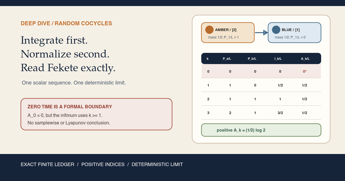
Begin with two states and calculate every finite value
Let the base space have two points:
\[ \Omega=\{\mathsf{amber},\mathsf{blue}\}. \]The base map swaps them:
\[ T(\mathsf{amber})=\mathsf{blue}, \qquad T(\mathsf{blue})=\mathsf{amber}. \]Give each point mass \(1/2\). This particular \(\mu\) is a probability measure , and the swap preserves it. The checked project theorem does not require probability; we choose it here because its two-value average is explicit.
Use one-dimensional complex matrices:
\[ A(\mathsf{amber})=[2], \qquad A(\mathsf{blue})=[1]. \]For a one-by-one matrix, the project’s maximum absolute row-sum norm is just the absolute value of its entry. Put
\[ L=\log 2\gt0. \]The finite log-positive cocycle observable is
\[ P_k(\omega)=\log^+\lVert C(k,\omega)\rVert_\infty. \]Starting at amber, the sampled factors are \(2,1,2,1,\ldots\). Starting at blue, they are \(1,2,1,2,\ldots\). Every factor has norm at least one, so positive log does not clip anything in this example:
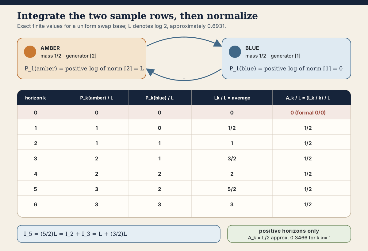
\[ \begin{aligned} P_k(\mathsf{amber})&=\left\lceil\frac{k}{2}\right\rceil L,\\ P_k(\mathsf{blue})&=\left\lfloor\frac{k}{2}\right\rfloor L. \end{aligned} \]Integrate the two values using their masses:
\[ \begin{aligned} I_k &= \int_\Omega P_k(\omega)\,d\mu(\omega)\\ &= \frac12P_k(\mathsf{amber}) +\frac12P_k(\mathsf{blue})\\ &= \frac{k}{2}L. \end{aligned} \]For positive \(k\), normalize:
\[ A_k=\frac{I_k}{k}=\frac12L\approx0.3466. \]Here is the complete horizon-zero-through-six ledger.
| \(k\) | \(P_k(\mathsf{amber})/L\) | \(P_k(\mathsf{blue})/L\) | \(I_k/L\) | \(A_k/L\) |
|---|---|---|---|---|
| 0 | 0 | 0 | 0 | \(0\), by Lean’s formal \(0/0=0\) convention |
| 1 | 1 | 0 | \(1/2\) | \(1/2\) |
| 2 | 1 | 1 | \(1\) | \(1/2\) |
| 3 | 2 | 1 | \(3/2\) | \(1/2\) |
| 4 | 2 | 2 | \(2\) | \(1/2\) |
| 5 | 3 | 2 | \(5/2\) | \(1/2\) |
| 6 | 3 | 3 | \(3\) | \(1/2\) |
The integrated sequence is not merely subadditive here; it is additive. For the split \(5=2+3\),
\[ I_5=\frac52L=I_2+I_3=L+\frac32L. \]That calculation is the finite arithmetic behind the general inequality \(I_{m+k}\le I_m+I_k\).
Boundary case: zero time can corrupt the infimum
Lean’s real division is total, so
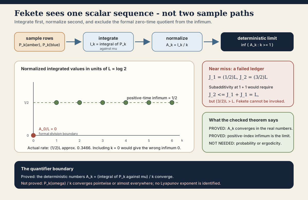
\[ A_0=\frac{I_0}{0}=\frac00=0. \]But the genuine positive-time values are \(L/2\gt0\). If we incorrectly took the infimum over all natural indices, the answer in this example would be zero. Mathlib’s Fekete limit instead uses indices \(k\ge1\), so its infimum is the correct value \(L/2\).
Near miss: a finite ledger that is not subadditive
Keep \(J_0=0\), but propose
\[ J_1=\frac12L, \qquad J_2=\frac32L. \]Subadditivity at \(1+1\) would require
\[ J_2\le J_1+J_1=L. \]Because \(L\gt0\), we instead have \(J_2=(3/2)L\gt L\). This candidate fails before any limit argument begins. A sequence does not become a Fekete sequence merely because its first few normalized values look bounded.
Name the objects before climbing
The chapter uses three different kinds of object:
| Symbol | Human meaning | Type after fixing the other inputs |
|---|---|---|
| \(P_k(\omega)\) | Finite log-positive growth at one outcome | \(\Omega\to\mathbb R\) |
| \(I_k\) | Integral of the entire outcome function | \(\mathbb R\) |
| \(A_k\) | Time-normalized integrated value | \(\mathbb R\) |
In Lean they are:
| Mathematics | Exact Lean expression |
|---|---|
| \(P_k(\omega)\) | C.logPlusNormObservable k ω |
| \(I_k\) | C.integratedLogPlusNorm k |
| \(A_k\) | C.normalizedIntegratedLogPlusNorm k |
The checked route is
\[ P_k(\omega) \longrightarrow I_k \longrightarrow A_k \longrightarrow \lim_{k\to\infty}A_k. \]The unproved route is
\[ P_k(\omega) \longrightarrow \frac{P_k(\omega)}{k} \longrightarrow \text{a limit depending on }\omega. \]Those arrows differ in both type and quantifier order. A limit of integrals is not automatically an integral of a limit, and neither is automatically an almost-everywhere statement. An almost-everywhere theorem would need a specified null set outside which samplewise convergence holds. No such set occurs in this module.
What the one-step hypothesis means
The predecessor chapter defined
C.HasIntegrableGeneratorLogPlus
as exactly
Integrable (C.logPlusNormObservable 1) μ
The word integrable means more than measurable : the real-valued function must also have finite integral of its norm. RMT-15 propagates that one-step hypothesis to every fixed finite horizon and to every finite orbit sum.
It does not require \(\mu(\Omega)=1\). Consequently, the project calls \(I_k\) an integral, not an expectation. In the two-point running example only, our chosen \(\mu\) is probabilistic, so \(I_k\) can also be read as an expectation .
Choose a route up
| Route | Begin with | Destination |
|---|---|---|
| Concrete route | The two-state ledger | Compute every displayed value before seeing an abstract integral |
| Type route | Name the objects | Keep functions of outcomes separate from deterministic numbers |
| Analytic route | Camp one | Learn why a real integral term is not itself a finiteness proof |
| Dynamics route | Camp two | See where measure preservation, rather than independence, enters |
| Algebra route | Camp four | Follow the pointwise cocycle split into scalar subadditivity |
| Limit route | The summit | Read the positive-index infimum and deterministic convergence exactly |
| Hands-on Lean route | Run the finite worksheet | Check the numeric ledger with only Lean core and Std |
| Audit route | The declaration map | Match every public source declaration to its role and assumptions |
Learning objectives
By the summit, you should be able to:
- reproduce the two-state sample and integral ledger through horizon six;
- explain why the swap preserves the uniform measure;
- distinguish \(P_k(\omega)\), \(I_k\), and \(A_k\) by type;
- explain why the running example is probabilistic although the theorem is stated for a raw measure;
- state the one-step integrability hypothesis exactly;
- explain Mathlib’s totalized Bochner-integral boundary;
- read the integrated time-zero and nonnegativity theorems without inferring hidden integrability;
- remove a base shift under an integral using measure preservation;
- distinguish preservation from independence and ergodicity;
- integrate the finite orbit sum and derive \(I_k\le kI_1\);
- derive \(I_{m+k}\le I_m+I_k\) in the correct block order;
- read
Subadditive C.integratedLogPlusNorm; - explain why \(A_0=0\) is not a zero-time growth rate;
- identify the positive-index set inside
Subadditive.lim; - explain why normalized ratios need not be monotone;
- run a bounded
Stdworksheet on a normal macOS or Linux host; - run the exact full project check with the pinned dependencies; and
- state why the result is neither samplewise nor a Lyapunov exponent.
Camp one: a totalized integral needs an integrability ledger
Declarations 1–3: define, evaluate zero time, and prove nonnegativity
The first definition is:
def integratedLogPlusNorm
    (C : DiscreteMatrixCocycle (ι := ι) μ) (k : ℕ) : ℝ :=
  ∫ ω, C.logPlusNormObservable k ω ∂μ
In Lean: integrate the whole outcome function
∫ ω, C.logPlusNormObservable k ω ∂μ∫ ω, … ∂μis Mathlib notation for the Bochner integral with bound variableωand measureμ.C.logPlusNormObservable kis a function \(\Omega\to\mathbb R\), not a scalar sample.- Appending
ωevaluates that function at one outcome inside the integrand. - The result is a single real number because the outcome variable is bound by the integral.
- The exact project definition is
DiscreteMatrixCocycle.integratedLogPlusNorm. - No
hCappears in the definition; that is a totality convention, not proof of integrability.
Mathlib’s Bochner integral is a total function. If a function is not
integrable, its totalized integral is defined to be zero. This design lets
integratedLogPlusNorm return a real number at every horizon even
before an integrability proof is supplied.
The stress test is the constant function one on an infinite-measure space. It is measurable but not integrable. Its totalized Bochner integral is still the real number zero. Therefore:
“Lean produced an \(\mathbb R\)” does not mean “the mathematical integral is finite.”
The source then proves
\[ I_0=0. \]RMT-15 already established \(P_0(\omega)=0\), including empty matrix dimension. Integrating the zero function closes the result.
It also proves
\[ 0\le I_k. \]Pointwise log-positive values are nonnegative, and
integral_nonneg transports that order to the totalized integral.
This theorem is unconditional. In a nonintegrable branch, it can say only
\(0\le0\), because totalization supplied the zero value.
Camp two: preservation removes a base shift after integration
Declaration 4: the pullback integral identity
The cocycle split contains a shifted later block:
\[ P_k(T^j\omega). \]Every natural iterate \(T^j\) preserves \(\mu\), so the module proves
\[ \int_\Omega P_k(T^j\omega)\,d\mu(\omega)=I_k. \]In Lean: erase a preserved shift only under the integral
C.integral_logPlusNormObservable_at_base_iterate_eq k jC.base^[j]in the theorem statement is the \(j\)-fold function iterate of the base map.C.base_iterate_preserving jsupplies both measurability of that iterate and the equality \(\operatorname{Measure.map}(T^j)\mu=\mu\).integral_mapconverts the pullback integral into an integral against the mapped measure.- Rewriting by
map_eqreturns the original measure. - The result removes the shift after integration. It does not prove \(P_k(T^j\omega)=P_k(\omega)\) pointwise.
- The exact theorem has no
hCargument because its totalized integral identity remains valid in the nonintegrable branch.
In the running example, \(T\) exchanges the two sample values. The uniform average is unchanged:
\[ \frac12P_k(\mathsf{blue})+\frac12P_k(\mathsf{amber}) =\frac12P_k(\mathsf{amber})+\frac12P_k(\mathsf{blue}). \]This is preservation, not independence. The two time samples are determined by the same starting state. It is also not ergodicity : the source needs only the stored measure-preserving interface.
Camp three: integrate the one-step orbit majorant
Declaration 5: the exact orbit-sum integral
RMT-15 defined
\[ S_k(\omega)=\sum_{j=0}^{k-1}P_1(T^j\omega). \]Under hC, every shifted one-step summand is integrable. Finite
linearity and the preserved-shift identity give
The checked theorem is
hC.integral_orbitLogPlusSum_eq k
At \(k=0\), the finite sum is empty and both sides are zero. No independence assumption appears: finite additivity of the integral and equality of each shifted integral are enough.
For the two-state example, \(S_k=P_k\) because each scalar factor has norm at least one. Its one-step integral is \(I_1=L/2\), so the equality reads
\[ \int_\Omega S_k\,d\mu=k\frac{L}{2}. \]In a general matrix cocycle, \(S_k\) can strictly overestimate \(P_k\). Positive log clips contraction at each step, and the norm inequality can lose additional information.
Declaration 6: the linear finite-horizon bound
RMT-15 proved the pointwise domination
\[ P_k(\omega)\le S_k(\omega). \]Both functions are integrable under hC. Integral monotonicity and
the exact orbit-sum calculation yield
This is a finite-horizon bound. For \(k\gt0\), it implies the derived estimate \(A_k\le I_1\), but the module does not export that specialization as another public declaration.
Camp four: build one subadditive real sequence
Declarations 7–8: integrate the cocycle split and package it
The pointwise finite-time theorem from RMT-15 is
\[ P_{m+k}(\omega) \le P_k(T^m\omega)+P_m(\omega). \]Notice the order:
- the early block has length \(m\) and begins at \(\omega\);
- the later block has length \(k\) and begins at \(T^m\omega\).
Under hC, every function in this inequality is integrable. The
proof applies integral monotonicity, expands the integral of the sum, and then
uses preservation to remove the shift:
The final commutation is addition of real numbers. It does not reverse or commute the underlying matrix factors.
In Lean: state scalar subadditivity at two horizons
C.integratedLogPlusNorm (m + k) ≤ C.integratedLogPlusNorm m + C.integratedLogPlusNorm km + kadds natural-number horizons.- Each
C.integratedLogPlusNorm …is now a deterministic real number; no outcome variable remains. ≤comes from the pointwise norm and positive-log inequalities, then integral monotonicity.- The proof needs
hCto justify integrability of all finite observables and the shifted term. - The exact theorem is
hC.integratedLogPlusNorm_add_le m k. - The wrapper
hC.subadditive_integratedLogPlusNormpackages the same statement asSubadditive C.integratedLogPlusNorm.
Mathlib defines
def Subadditive (u : ℕ → ℝ) : Prop :=
  ∀ m n, u (m + n) ≤ u m + u n
At this line, the dynamical problem has been reduced to a deterministic sequence problem. Fekete will see the function
C.integratedLogPlusNorm : ℕ → ℝ
and the subadditivity proof. It will not see \(\omega\), the base map, the generator, or a sample path.
Why the near miss is rejected here
For \(J_1=L/2\) and \(J_2=3L/2\), Lean would need the false inequality
\[ \frac32L\le\frac12L+\frac12L. \]No amount of lower boundedness or numerical plotting repairs that missing subadditivity proof. The theorem’s hypothesis is structural, not empirical.
Camp five: normalize positive time and totalize horizon zero
Declarations 9–11: normalized values, nonnegativity, and a lower bound
The source defines:
def normalizedIntegratedLogPlusNorm
    (C : DiscreteMatrixCocycle (ι := ι) μ) (k : ℕ) : ℝ :=
  C.integratedLogPlusNorm k / k
In Lean: divide the integrated scalar by elapsed time
C.integratedLogPlusNorm k / k- The numerator is a real number.
- The denominator
kbegins as a natural number and is coerced to \(\mathbb R\) because real division is expected. - The slash is real division, not natural-number division.
- At
k = 0, the result is total and equals zero. - The definition contains no outcome variable, so it is not the samplewise
quantity
C.logPlusNormObservable k ω / k. - The exact project name is
normalizedIntegratedLogPlusNorm.
Nonnegativity of \(I_k\) and of the coerced natural denominator gives
\[ 0\le A_k \]for every \(k\), including zero. The source then proves
\[ \operatorname{BddBelow}(\operatorname{range} A) \]by exhibiting zero as a lower bound.
This lower-bound proof is unconditional because it is an order theorem about
the totalized values. The later Fekete rate still takes hC,
because its subadditivity proof depends on finite-horizon integrability.
Summit: read Mathlib’s Fekete limit literally
Declaration 12: define the positive-index infimum
The project rate is:
def integratedLogPlusGrowthRate
    (C : DiscreteMatrixCocycle (ι := ι) μ)
    (hC : C.HasIntegrableGeneratorLogPlus) : ℝ :=
  hC.subadditive_integratedLogPlusNorm.lim
In Lean: use the limit attached to the subadditivity proof
hC.subadditive_integratedLogPlusNorm.limhCis the one-step integrability proof..subadditive_integratedLogPlusNormturns it into a proof that the scalar sequence \(I_k\) is subadditive..limis Mathlib’s protected definition in theSubadditivenamespace.- In the pinned Mathlib source, it unfolds to
sInf ((fun n : ℕ => u n / n) ’’ Set.Ici 1). Set.Ici 1means the natural indices \(n\ge1\); zero is absent.sInfis an infimum. The definition does not claim that one finite horizon attains it.
Thus the exact semantics are
\[ \gamma_\mu^+(C) =\inf\left\{\frac{I_k}{k}:k\in\mathbb N,\ k\ge1\right\}. \]The superscript \(+\) is expository notation for this page. The Lean source
name is integratedLogPlusGrowthRate. The positive sign reminds us
that the underlying observable uses \(\log^+\) and therefore discards
contraction and singular collapse.
Declaration 13: deterministic convergence
The final theorem is:
theorem HasIntegrableGeneratorLogPlus.tendsto_normalizedIntegratedLogPlusNorm
    {C : DiscreteMatrixCocycle (ι := ι) μ}
    (hC : C.HasIntegrableGeneratorLogPlus) :
    Tendsto C.normalizedIntegratedLogPlusNorm atTop
      (𝓝 (C.integratedLogPlusGrowthRate hC))
In Lean: say that the scalar sequence converges
Tendsto C.normalizedIntegratedLogPlusNorm atTop (𝓝 (C.integratedLogPlusGrowthRate hC))Tendstois a filter-based convergence statement.C.normalizedIntegratedLogPlusNormis the deterministic function \(\mathbb N\to\mathbb R\).atTopexpresses \(k\to\infty\) in natural time.𝓝 xis the neighborhood filter of the real numberx.- The target is exactly the rate defined from
Subadditive.lim. - There is no
ω,∀ᵐ ω ∂μ, exceptional set, random variable, convergence-in-probability predicate, or \(L^1\) norm in the theorem.
The proof calls Mathlib’s deterministic
Subadditive.tendsto_lim with two inputs:
- scalar subadditivity obtained from
hC; and - the unconditional zero lower bound for the normalized range.
That is the whole asymptotic engine.
Fekete ratios need not decrease
Fekete convergence does not say \(u_n/n\) is monotone. A simple calibration sequence is
\[ u_n=\left\lceil\frac n2\right\rceil. \]It is subadditive because
\[ \left\lceil\frac{m+n}{2}\right\rceil \le \left\lceil\frac m2\right\rceil +\left\lceil\frac n2\right\rceil. \]Its positive ratios begin
\[ 1,\quad \frac12,\quad \frac23,\quad \frac12,\quad \frac35,\quad \frac12,\ldots \]They rise and fall while converging to \(1/2\). Therefore the correct phrase is “converges to the infimum,” not “decreases to the infimum.”
Type the finite ledger yourself with Lean and Std
The project theorem imports Mathlib’s matrices, measure theory, integration,
and subadditive analysis. The opening arithmetic does not need that entire
dependency graph. The worksheet below imports only Lean’s Std
library.
It measures sample values in units of \(L=\log 2\). To avoid implementing real integration in a toy file,
integratedNumerator k = 2 I_k / L.
For the uniform two-point measure, that numerator equals \(k\). The worksheet checks the two finite rows, the integrated numerator, an additive split, the formal zero boundary, and the failed near miss.
This is a standalone tutorial. It is suitable for an ordinary macOS or Linux host and does not invoke Lake, Mathlib, or a project build.
Save the exact block below as
/tmp/IntegratedLogPlusFeketeTutorial.lean:
import Std

namespace IntegratedLogPlusFeketeTutorial

inductive State where
  | amber
  | blue
  deriving Repr, DecidableEq

def base : State → State
  | .amber => .blue
  | .blue => .amber

/-- `sampleLogUnits k ω` is the finite log-positive value in units of `log 2`. -/
def sampleLogUnits : Nat → State → Nat
  | 0, _ => 0
  | k + 1, .amber => sampleLogUnits k .blue + 1
  | k + 1, .blue => sampleLogUnits k .amber

/-- Twice the uniform integral, still measured in units of `log 2`. -/
def integratedNumerator (k : Nat) : Nat :=
  sampleLogUnits k .amber + sampleLogUnits k .blue

theorem integratedNumerator_eq (k : Nat) :
    integratedNumerator k = k := by
  induction k with
  | zero => rfl
  | succ k ih =>
      simpa [integratedNumerator, sampleLogUnits, Nat.add_assoc,
        Nat.add_comm, Nat.add_left_comm] using congrArg Nat.succ ih

theorem integratedNumerator_add (m k : Nat) :
    integratedNumerator (m + k) =
      integratedNumerator m + integratedNumerator k := by
  simp [integratedNumerator_eq]

/-- The normalized numerator. At zero, natural-number division returns zero. -/
def normalizedNumerator (k : Nat) : Nat :=
  integratedNumerator k / k

theorem normalizedNumerator_eq_one {k : Nat} (hk : 0 < k) :
    normalizedNumerator k = 1 := by
  rw [normalizedNumerator, integratedNumerator_eq]
  exact Nat.div_self hk

/-- A candidate ledger that fails subadditivity already at one plus one. -/
def nearMiss : Nat → Nat
  | 0 => 0
  | 1 => 1
  | 2 => 3
  | k + 3 => k + 3

#eval (List.range 7).map fun k =>
  (k, sampleLogUnits k .amber, sampleLogUnits k .blue,
    integratedNumerator k, normalizedNumerator k)

#eval decide
  (integratedNumerator 5 =
    integratedNumerator 2 + integratedNumerator 3)

#eval decide (nearMiss 2 ≤ nearMiss 1 + nearMiss 1)

example : normalizedNumerator 0 = 0 := by decide
example : integratedNumerator 6 = 6 := by decide
example : integratedNumerator 5 =
    integratedNumerator 2 + integratedNumerator 3 := by decide
example : ¬ nearMiss 2 ≤ nearMiss 1 + nearMiss 1 := by decide

end IntegratedLogPlusFeketeTutorial
Open a terminal and type:
source "$HOME/.elan/env"
elan run leanprover/lean4:v4.32.0 lean \
  /tmp/IntegratedLogPlusFeketeTutorial.lean
The exact worksheet above was executed successfully with Lean 4.32.0 while editing this chapter. Its output was:
[(0, 0, 0, 0, 0), (1, 1, 0, 1, 1), (2, 1, 1, 2, 1), (3, 2, 1, 3, 1), (4, 2, 2, 4, 1), (5, 3, 2, 5, 1), (6, 3, 3, 6, 1)]
true
false
Each five-tuple is
(k, amber sample, blue sample, integrated numerator, normalized numerator).
- The first line reproduces horizons zero through six.
- At positive horizons the final coordinate is one. Translating out of the doubled units gives \(A_k/L=1/2\).
- The first
truechecks the exact split \(I_5=I_2+I_3\) after multiplying all values by \(2/L\). - The final
falsechecks that the near miss does not satisfy its \(1+1\) subadditivity test. - The silent
exampledeclarations give kernel-checked proofs of the zero boundary, the horizon-six value, the additive split, and the negation of the near-miss inequality.
The worksheet is a finite model, not the project theorem. It uses natural counts instead of real logarithms, encodes the uniform two-point integral by a sum and a known factor \(1/2\), and proves no statement about arbitrary measures, Bochner integrals, matrices, measurable maps, integrability, subadditive real sequences, or limits. Its job is to make the page’s opening numbers executable on a modest computer.
The complete thirteen-declaration map
The source module exposes exactly thirteen public declarations.
| # | Declaration | Needs hC? | Exact role |
|---|---|---|---|
| 1 | integratedLogPlusNorm | No | Totalized real integral of the finite log-positive observable |
| 2 | integratedLogPlusNorm_zero | No | The integrated time-zero value is zero |
| 3 | integratedLogPlusNorm_nonneg | No | Every totalized integrated value is nonnegative |
| 4 | integral_logPlusNormObservable_at_base_iterate_eq | No | A preserved finite base shift leaves the totalized integral unchanged |
| 5 | HasIntegrableGeneratorLogPlus.integral_orbitLogPlusSum_eq | Yes | The finite one-step orbit-sum integral equals \(kI_1\) |
| 6 | HasIntegrableGeneratorLogPlus.integratedLogPlusNorm_le_nat_mul | Yes | \(I_k\le kI_1\) |
| 7 | HasIntegrableGeneratorLogPlus.integratedLogPlusNorm_add_le | Yes | \(I_{m+k}\le I_m+I_k\) |
| 8 | HasIntegrableGeneratorLogPlus.subadditive_integratedLogPlusNorm | Yes | Packages declaration 7 as Mathlib’s Subadditive predicate |
| 9 | normalizedIntegratedLogPlusNorm | No | Defines the total natural-time ratio \(A_k=I_k/k\) |
| 10 | normalizedIntegratedLogPlusNorm_nonneg | No | Every normalized totalized value is nonnegative |
| 11 | bddBelow_normalizedIntegratedLogPlusNorm | No | Zero bounds the full normalized range from below |
| 12 | integratedLogPlusGrowthRate | Yes | Names the positive-index Fekete infimum |
| 13 | HasIntegrableGeneratorLogPlus.tendsto_normalizedIntegratedLogPlusNorm | Yes | Proves deterministic real convergence to that infimum |
The assumption ledger is just as important:
| Data or property | Present? | Consequence |
|---|---|---|
| Measurable base space | Yes | Observables and pullbacks can enter measure theory |
| Finite matrix index type with decidable equality | Yes | Finite complex matrices and their norm are available |
| Arbitrary measure \(\mu\) | Yes | Integrals are raw measure integrals by default |
| Base preserves \(\mu\) | Yes | Shifted pullback integrals agree |
| Measurable generator | Yes | Finite observables are measurable |
One-step log-positive integrability hC | Required for declarations 5–8 and 12–13 | Finite integral algebra and scalar subadditivity are justified |
| Probability normalization | No | “Expectation” is not the general theorem’s terminology |
| Ergodicity, mixing, or independence | No | No orbit-average or decorrelation conclusion follows |
| Invertibility | No | Time remains one-sided |
| Negative-log control | No | Contraction and collapse are not recovered |
Empty matrix dimension
The index type may be empty. RMT-15 proves that every log-positive norm observable is then the zero function. The one-step hypothesis is satisfied, all integrated and normalized values are zero, and the deterministic Fekete rate is zero.
That boundary is consistent, but it does not explain positive-dimensional growth. It records that the envelope has no coordinates from which to collect growth.
Raw measure scaling
In the opening example, replacing the uniform probability measure \((1/2,1/2)\) with counting measure \((1,1)\) doubles every integral:
\[ I_k^{\mathrm{count}}=kL, \qquad A_k^{\mathrm{count}}=L. \]The cocycle did not change; the measure normalization did. This is why the general symbol \(\gamma_\mu^+(C)\) should remember \(\mu\), and why the source does not call its raw integral an expectation.
Common wrong turns
Calling \(I_k\) an expectation for an arbitrary measure
An expectation requires a probability measure. The module assumes only a measure. Say “integral” unless a probability instance is explicitly in scope.
Treating a totalized real integral as an integrability proof
The Bochner integral has a real value even when the integrand is
nonintegrable. Use the explicit hC propagation theorem.
Deleting the base shift pointwise
Preservation proves equal integrals of \(P_k\circ T^m\) and \(P_k\). It does not prove those functions are equal at each outcome.
Reading preservation as independence
All orbit observables can be functions of the same initial outcome. Equal shifted integrals do not factor a joint law.
Including \(A_0\) in the Fekete infimum
The running example gives a direct counterexample: \(A_0=0\), but every
positive value is \(L/2\). Mathlib uses Set.Ici 1.
Saying the ratios decrease
Fekete gives convergence to an infimum. The ratios may oscillate, as \(\lceil n/2\rceil/n\) does.
Replacing the rate by \(I_1\)
The bound \(I_k\le kI_1\) implies \(\gamma_\mu^+(C)\le I_1\). It does not generally imply equality. The running example happens to have equality \(A_k=I_1=L/2\) because its integrated sequence is additive.
Moving a limit through the integral
The theorem takes a limit of the scalars \(\int P_k\,d\mu/k\). It proves no pointwise limit and no dominated- or uniform-integrability hypothesis that would justify interchanging limit and integral.
Calling the conclusion a Lyapunov exponent
A Lyapunov exponent normally records samplewise exponential growth and is sensitive to contraction. This module integrates first and uses \(\log^+\), which clips all nonpositive logarithmic growth.
Invoking Kingman retroactively
The proof invokes deterministic Fekete convergence, not a subadditive ergodic theorem. No almost-sure convergence theorem occurs in the source.
Exercises from trailhead to summit
Trailhead
- Starting from amber, multiply the first six one-by-one generator matrices and recover the first sample row.
- Repeat from blue.
- Average the two rows and verify \(I_k=(k/2)L\).
- Explain in one sentence why the uniform swap measure is preserved.
- Compute the same integral with counting measure.
- Identify the first horizon at which the two sample values agree.
Mid-mountain
- Prove on paper that \(\lceil k/2\rceil+\lfloor k/2\rfloor=k\).
- Verify \(I_{m+k}=I_m+I_k\) for the running example.
- Show exactly where the near-miss ledger fails subadditivity.
- Construct another finite sequence that passes the \(1+1\) test but fails a later subadditivity test.
- Explain why
integratedLogPlusNorm_nonnegdoes not prove integrability. - Trace the shifted \(k\)-block through the proof of
integratedLogPlusNorm_add_le. - Explain why finite integral additivity needs the propagated integrability proofs.
- Show that \(I_k\le kI_1\) does not force \(I_k=kI_1\).
Summit
- Unfold
Subadditive.limin the pinned Mathlib source and point to the positive-index restriction. - Prove that \(u_n=\lceil n/2\rceil\) is subadditive and that its ratios are not monotone.
- State a candidate samplewise theorem using an explicit almost-everywhere quantifier. List every new hypothesis it would need.
- Explain why convergence of \(I_k/k\) alone does not imply convergence of \(P_k(\omega)/k\).
- Explain what contraction information \(\log^+\) discards for a scalar factor \(a\) with \(0\lt|a|\lt1\).
- Design a collapse-sensitive observable for a zero scalar factor and state the codomain problem it introduces.
- Compare the deterministic Fekete conclusion with the statement of a subadditive ergodic theorem, keeping hypotheses and quantifiers separate.
Inspect and check the exact project interfaces
The authoritative source is
formalization/NonlinearDynamics/Random/RandomCocycles/IntegratedLogPlusGrowth.lean.
For a full project check, install the repository’s pinned dependencies and
place the following in a temporary project scratch file:
import NonlinearDynamics.Random.RandomCocycles.IntegratedLogPlusGrowth

open Matrix MeasureTheory Set Filter Topology
open scoped Matrix.Norms.Operator Real
open NonlinearDynamics.Random.RandomCocycles

#check DiscreteMatrixCocycle.integratedLogPlusNorm
#check DiscreteMatrixCocycle.integratedLogPlusNorm_zero
#check DiscreteMatrixCocycle.integratedLogPlusNorm_nonneg
#check DiscreteMatrixCocycle.integral_logPlusNormObservable_at_base_iterate_eq
#check DiscreteMatrixCocycle.HasIntegrableGeneratorLogPlus.integral_orbitLogPlusSum_eq
#check DiscreteMatrixCocycle.HasIntegrableGeneratorLogPlus.integratedLogPlusNorm_le_nat_mul
#check DiscreteMatrixCocycle.HasIntegrableGeneratorLogPlus.integratedLogPlusNorm_add_le
#check DiscreteMatrixCocycle.HasIntegrableGeneratorLogPlus.subadditive_integratedLogPlusNorm
#check DiscreteMatrixCocycle.normalizedIntegratedLogPlusNorm
#check DiscreteMatrixCocycle.normalizedIntegratedLogPlusNorm_nonneg
#check DiscreteMatrixCocycle.bddBelow_normalizedIntegratedLogPlusNorm
#check DiscreteMatrixCocycle.integratedLogPlusGrowthRate
#check DiscreteMatrixCocycle.HasIntegrableGeneratorLogPlus.tendsto_normalizedIntegratedLogPlusNorm
The #check commands report existing declaration
types. They do not create a samplewise exponent, prove an ergodic theorem, or
replace the source module’s compilation.
From the repository root, the exact command is:
cd formalization
lake env lean NonlinearDynamics/Random/RandomCocycles/IntegratedLogPlusGrowth.lean
This full project check may compile substantial dependencies and therefore may require substantial disk space and memory.
cd formalization
lake env lean -DwarningAsError=true NonlinearDynamics/Random/RandomCocycles/IntegratedLogPlusGrowth.lean
Resource note: this exact file uses the repository's
pinned Lean and Mathlib dependencies. Initial project setup can require
substantial disk space and build time. For a lightweight first step on
macOS or Linux, use the page's standalone Lean-core or Std
tutorial.
Technical success does not complete human or Pro review.
What the checked theorem does and does not say
| Topic | Status in this module |
|---|---|
| Finite-horizon log-positive integral | Defined as a total real value |
| Integrated time-zero value | Proved zero |
| Integrated nonnegativity | Proved without claiming integrability |
| Shifted pullback integral | Proved invariant under every preserved base iterate |
| One-step integrability hypothesis | Inherited explicitly from RMT-15 |
| Exact finite orbit-sum integral | Proved under hC |
| Linear bound \(I_k\le kI_1\) | Proved under hC |
| Scalar subadditivity | Proved under hC |
| Natural-time normalization | Defined, including formal time zero |
| Lower bound | Zero bounds the full normalized range |
| Rate | Defined as Mathlib’s positive-index Fekete infimum |
| Deterministic convergence | Proved in \(\mathbb R\) |
| Probability normalization | Not assumed |
| Finite total measure | Not assumed |
| Independence, mixing, or ergodicity | Not assumed or proved |
| Monotonic normalized ratios | Not implied |
| Pointwise or almost-sure convergence | Not proved |
| Convergence in probability, distribution, or \(L^1\) | Not proved |
| Limit-integral interchange | Not attempted |
| Kingman’s subadditive ergodic theorem | Not invoked |
| Furstenberg–Kesten theorem | Not invoked |
| Contraction-sensitive logarithmic rate | Not available from \(\log^+\) |
| Lyapunov exponent or spectrum | Not defined or proved |
| Oseledets filtration or splitting | Not invoked |
| Two-sided cocycle or inverse estimates | Not present |
| Random Jacobian interpretation | Not connected |
The exact summit is narrower:
One-step integrability plus measure preservation turns the finite log-positive cocycle envelope into a lower-bounded subadditive sequence of real integrals. Its positive-time normalized values converge to their deterministic Fekete infimum.
No outcome-dependent limit appears in that sentence.
Where to continue
Finite-Horizon Log-Positive Cocycle Integrability
is the immediate predecessor. It constructs \(P_k\), the finite orbit sum,
and the propagated hC proofs used here.
Probability Normalization and Ergodic Rigidity Before Kingman is the immediate successor. It adds a probability-specialized interface and native ergodic rigidity while still refusing to claim a samplewise limit.
The compact integrated log-positive growth rate glossary entry is the quick reference for the rate and its caveats.
Integrated Log-Positive Growth in Lean: Subadditivity and a Deterministic Fekete Limit is the paired Development Notebook entry.
A genuine Lyapunov chapter must choose additional mathematics rather than renaming this result. At minimum it must decide:
- the samplewise convergence theorem and its exact quantifiers;
- probability or finite-measure normalization;
- the required subadditive-process measurability and integrability hypotheses;
- how contraction and zero matrices are represented;
- whether the cocycle is one-sided or invertible; and
- whether the target is one exponent, all singular-value exponents, or an invariant filtration or splitting.
References
Nonlinear Dynamics in Lean. IntegratedLogPlusGrowth.lean. This is the authoritative thirteen-declaration project source described by the chapter.
Mathlib contributors.
Subadditive and superadditive sequences,
Mathlib 4 documentation. The pinned source defines
Subadditive, the positive-index Subadditive.lim, and
the lower-bounded deterministic convergence theorem used here.
Mathlib contributors. The Bochner integral, Mathlib 4 documentation. This official source documents the totalized integral and the integral operations used by the module.
Mathlib contributors. Measure-preserving maps, Mathlib 4 documentation. This is the upstream interface for mapped-measure equality, natural iterates, and pullback integrability.
M. Fekete. Über die Verteilung der Wurzeln bei gewissen algebraischen Gleichungen mit ganzzahligen Koeffizienten, Mathematische Zeitschrift 17, 228–249, 1923. This is the historical primary source associated with the deterministic subadditive lemma.
Harry Furstenberg and Harry Kesten. Products of Random Matrices, The Annals of Mathematical Statistics 31(2), 457–469, 1960. This primary source motivates random-matrix-product growth. The present module proves none of its probabilistic or samplewise conclusions.
J. F. C. Kingman. The ergodic theory of subadditive stochastic processes, Journal of the Royal Statistical Society: Series B 30(3), 499–510, 1968. Kingman’s theorem has additional hypotheses and samplewise content. It is not invoked here.
V. I. Oseledets. A multiplicative ergodic theorem: characteristic Ljapunov exponents of dynamical systems, Transactions of the Moscow Mathematical Society 19, 197–231, 1968. This is a later exponent-and-splitting destination, not a result of the present module.
The exact upstream Lean source audited for this chapter is Mathlib commit
81a5d257,
the revision pinned by formalization/lake-manifest.json. The
project source file audited while rebuilding this page had SHA-256
e5ce3cb8cfdec22bae395be609b00a2ae7e17b3928b031005a1232d8c00eec57.