A calculation with all three signs
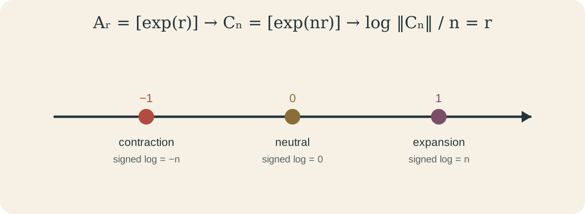
Let the sample space contain one point of mass one. Let the base map be the identity, and let the generator be the one-by-one matrix \(A_r=[e^r]\). For every natural horizon \(n\),
\[ C_n=A_r^n=[e^{nr}], \qquad \lVert C_n\rVert=e^{nr}, \qquad \log\lVert C_n\rVert=nr. \]At every positive horizon, division by \(n\) gives exactly \(r\). Choosing \(r=-1,0,1\) yields contraction, neutrality, and expansion. The probability space, generator, and observable are measurable; the forward and inverse one-step log-positive values are finite constants; and the generator is invertible because \(e^r\ne0\).
This calculation matters twice. It shows why the theorem must allow a negative answer, and it identifies what the general output should mean. It does not establish the theorem for nonconstant or noncommuting matrix products.
Four objects that must not be conflated
For a general cocycle, write
\[ X_n(\omega)=\log\lVert C_n(\omega)\rVert. \]There are four related objects:
- \(X_n(\omega)\), a finite-horizon sample value;
- \(X_n(\omega)/n\), a normalized sample value;
- \(a_n=\int X_n\,d\mu\), a deterministic signed integral; and
- \(\lambda=\lim_n a_n/n\), the deterministic integrated Fekete rate.
The almost-everywhere theorem identifies the limit of the second object with the fourth under the stated assumptions. It does not say that one may first take a sample limit and then integrate it. Such an interchange would require additional analysis absent from RMT-35.
The total real logarithm in Lean assigns a value at zero. RMT-34 therefore stores pointwise invertibility separately: every generator is a matrix unit, so every finite product is nonzero and ordinary signed logarithmic algebra is valid. The same hypothesis package asks that
\[ \log^+\lVert A(\omega)\rVert \quad\text{and}\quad \log^+\lVert A(\omega)^{-1}\rVert \]be integrable. The forward term controls expansion. The inverse term controls contraction.
Why the deterministic rate is finite
Signed subadditivity says
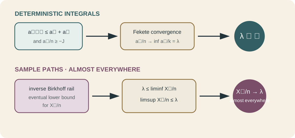
\[ X_{m+n}(\omega) \le X_m(\omega)+X_n(T^m\omega). \]Integrability allows the inequality to be integrated, and measure preservation turns the shifted second integral back into \(a_n\). Hence
\[ a_{m+n}\le a_m+a_n. \]Subadditivity alone could still lead toward negative infinity. The inverse tail supplies a finite linear floor:
\[ -nJ\le a_n, \qquad J=\int\log^+\lVert A(\omega)^{-1}\rVert\,d\mu(\omega). \]Therefore \(a_n/n\ge-J\) at every positive horizon. Mathlib’s real-valued Fekete theorem applies and produces a finite limit
\[ \lambda=\lim_{n\to\infty}\frac{a_n}{n} =\inf_{n\ge1}\frac{a_n}{n}. \]def integratedRealLogGrowthRate ... :=\n hC.subadditive_integratedRealLogNorm.lim\n\nhC.tendsto_normalizedIntegratedRealLogNorm\nhC.integratedRealLogGrowthRate_eq_sInfdef introduces the rate as data depending on the cocycle and its tail
hypothesis. The method .lim is Mathlib’s finite Fekete limit for a
subadditive real sequence whose normalized range is bounded below. Tendsto
states convergence; sInf states the positive-horizon infimum formula.Why the sample paths reach that rate
An integral limit does not automatically determine a sample limit. RMT-35 proves two almost-everywhere inequalities.
The lower-deviation machinery yields
\[ \lambda\le\liminf_n X_n(\omega)/n. \]The upper argument is more delicate. Earlier phase averaging was first packaged for nonnegative processes. Signed real logs are not nonnegative, so RMT-29 was generalized to ask for the actual analytic need: eventual boundedness below of the normalized path.
Pointwise invertibility gives the comparison
\[ -\frac1n\sum_{j=0}^{n-1} \log^+\lVert A(T^j\omega)^{-1}\rVert \le \frac{X_n(\omega)}n. \]The function on the left is the negative of a Birkhoff average of an integrable function. Pointwise Birkhoff convergence makes it bounded almost everywhere, so normalized signed growth is eventually bounded below there. The generalized phase-averaging result then gives
\[ \limsup_n X_n(\omega)/n\le\lambda. \]Since \(\liminf\le\limsup\), the two estimates force equality and convergence.
Reading the formal endpoint
theorem HasIntegrableGeneratorLogTails.ae_tendsto_normalizedRealLogNormObservable\n [IsProbabilityMeasure μ]\n (hC : C.HasIntegrableGeneratorLogTails)\n (hT : PreErgodic C.base μ) :\n ∀ᵐ ω ∂μ, Tendsto\n (fun n ↦ normalizedProcess C.realLogNormObservable n ω)\n atTop (𝓝 (C.integratedRealLogGrowthRate hC))∀ᵐ ω ∂μ means “for almost every ω with respect to μ.”
normalizedProcess divides the horizon-\(n\) observable by \(n\), with a
totalized value at zero. atTop sends \(n\) to infinity. 𝓝 is the
neighborhood filter of the real rate. PreErgodic is the invariant-set
rigidity assumption; preservation is already stored in the cocycle.The endpoint requires a probability measure, not merely an arbitrary finite measure, because its deterministic normalization and ergodic identification are stated in that setting. Empty matrix dimension is still legal and has rate zero. If the older log-positive rate is strictly positive, the signed and log-positive rates agree by uniqueness of almost-everywhere limits.
Try the two resource levels
For a standalone tutorial, save the following as SignedRateTutorial.lean.
It imports only Std and checks the integer model on macOS or Linux:
import Std

def signedPrefix (rate : Int) (n : Nat) : Int := (n : Int) * rate

example (n : Nat) : signedPrefix (-1) n = -(n : Int) := by
  simp [signedPrefix]

example (n : Nat) : signedPrefix 0 n = 0 := by
  simp [signedPrefix]

example (n : Nat) : signedPrefix 1 n = n := by
  simp [signedPrefix]
Run lean SignedRateTutorial.lean. This checks only the scalar arithmetic
analogy.
cd formalization
lake env lean -DwarningAsError=true NonlinearDynamics/Random/RandomCocycles/RealLogNormKingman.lean
Resource note: this exact file uses the repository's
pinned Lean and Mathlib dependencies. Initial project setup can require
substantial disk space and build time. For a lightweight first step on
macOS or Linux, use the page's standalone Lean-core or Std
tutorial.
Boundary audit
- Contraction: the private constant scalar model has exact rate \(-1\); this confirms that no nonnegativity premise entered the endpoint.
- Neutrality: the same model at rate zero checks the boundary between contraction and expansion.
- Expansion: rate \(1\) checks the positive regime where signed and positive-log growth agree.
- Time zero: normalized values are totalized, while every Fekete infimum and division argument uses positive horizons.
- Empty dimension: the public theorem records rate zero without assuming an inhabitant of the matrix index.
- Singular generators: excluded from the signed theorem by pointwise
invertibility. The total value
Real.log 0 = 0is not a substitute for signed logarithmic algebra at collapse.
What remains outside the theorem
The source proves almost-everywhere convergence only. It supplies no \(L^1\) convergence, uniform integrability of the normalized signed family, limit-integral interchange, rate of convergence, concentration inequality, conorm or singular-value limit, Lyapunov spectrum, invariant splitting, Oseledets theorem, derivative-cocycle theorem, or stable-manifold theorem. Those statements require additional definitions and hypotheses.
References
- J. F. C. Kingman, “The Ergodic Theory of Subadditive Stochastic Processes,” JRSS Series B 30(3), 499–510 (1968), publisher record and DOI.
- Signed Real-Log Kingman Convergence in Lean.
- Integrated real-log growth rate.
- The Forward-and-Inverse Tail Sandwich for Finite-Time Real Log Norms.