A countdown certificate
Begin with the update rule on natural numbers that subtracts one until zero:
\[ f(0)=0,\qquad f(n+1)=n. \]Take \(V(n)=n\). Then \(V(n)\ge0\), \(V(n)=0\) exactly when \(n=0\), and
\[ n\ne0\Longrightarrow V(f(n))\lt V(n). \]Every orbit reaches zero after finitely many steps. The bundled
countdown-energy.lean worksheet checks these finite algebraic statements
using Lean and Std. It is a model of the descent pattern, not a replacement
for the metric and topological hypotheses used by the project theorem.
The identity update supplies the nearest boundary. The same \(V\) weakly decreases because \(V(f(n))=V(n)\), but a positive start remains positive forever. Weak descent alone therefore cannot establish attraction.
The scalar difference
For a general self-map \(f:X\to X\) and scalar function \(V:X\to\mathbb R\), write
\[ \Delta V(x)=V(f(x))-V(x). \]The sign of this one-step difference describes scalar descent. It does not, by itself, define stability of the state.
def IsWeakLyapunovDecreaseOn\n (f : X → X) (V : X → ℝ) (S : Set X) : Prop :=\n ∀ x ∈ S, V (f x) ≤ V xS is part of the statement. ∀ x ∈ S restricts the estimate to
that region. Nothing in this definition says that f maps S back into
itself, so forward invariance remains a separate premise.Strict descent replaces ≤ by < away from the reference point. If the
reference is fixed, the strict condition implies weak descent: at the
reference point the scalar value is unchanged, and everywhere else strict
inequality can be weakened to non-strict inequality.
Why positivity has two levels
Nonnegative means \(V(x)\ge0\). Positive definite relative to \(p\) means
\[ V(p)=0,\qquad x\ne p\Longrightarrow V(x)\gt0. \]The second condition identifies one zero. The zero function satisfies the first condition everywhere and the second nowhere on a state space with more than one point. This distinction blocks a useless certificate from being treated as if it localized the reference state.
The project also distinguishes a selected region from a neighborhood-level
statement. IsPositiveDefiniteOn V p S carries S explicitly and requires
that p belongs to it.
IsLocallyPositiveDefiniteAt V p requires strict positivity away from p in
some neighborhood. A region certificate becomes local when S itself is a
neighborhood. Neither form claims a global basin.
Sublevels are the trapping device
For \(c\in\mathbb R\), an open sublevel is
\[ L_c=\{x:V(x)\lt c\}. \]If \(V(f(x))\le V(x)\), then \(x\in L_c\) implies \(f(x)\in L_c\). On a selected region \(S\), the proof also needs \(f(S)\subseteq S\). Repeating the one-step estimate gives
\[ V(f^{n+1}(x))\le V(f^n(x))\le V(x). \]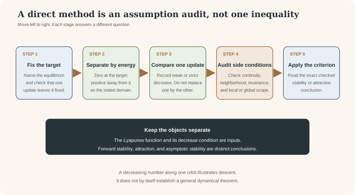
In Lean, Set.MapsTo f S S expresses forward invariance. The two sublevel
theorems preserve intersections with \(S\). iterate_le proves the bound by
induction, while antitone_orbit packages all pairwise time comparisons as an
Antitone sequence.
From trapping to stability
The missing geometry is expressed by HasSublevelControlAt V p:
This premise is deliberately stronger than pointwise positive definiteness. In finite-dimensional Euclidean proofs, compact annuli often produce the needed positive separation. An arbitrary pseudo-metric space offers no such compactness automatically.
If \(V(p)=0\) and \(V\) is continuous at \(p\), then every positive sublevel is
a neighborhood of \(p\). Choose a small initial ball inside it. Weak descent
keeps all iterates in the sublevel, and sublevel control keeps all iterates in
the requested epsilon ball. That is the checked theorem
isLyapunovStableFixedPoint_of_continuousAt_of_sublevelControl.
Notice the conclusion: Lyapunov stability says that starts sufficiently close to \(p\) remain close at every natural-number time. It does not say that their distance tends to zero.
Attraction is a separate limit
To obtain attraction, the first slice assumes the scalar conclusion directly:
\[ V(f^n(x))\to0. \]For any epsilon, sublevel control selects a positive threshold \(c\). The
scalar limit eventually places every later orbit value below \(c\), and the
control implication places every later state inside the epsilon ball. This is
isAttractedTo_of_tendsto_lyapunov.
Universal quantification over starts yields
isGloballyAttractingFixedPoint_of_tendsto_lyapunov. Combining the local
stability theorem with the universal limit yields
isAsymptoticallyStableFixedPoint_of_lyapunov. The API does not disguise a
global hypothesis as a local one: the universal scalar limit appears
literally in the theorem statement.
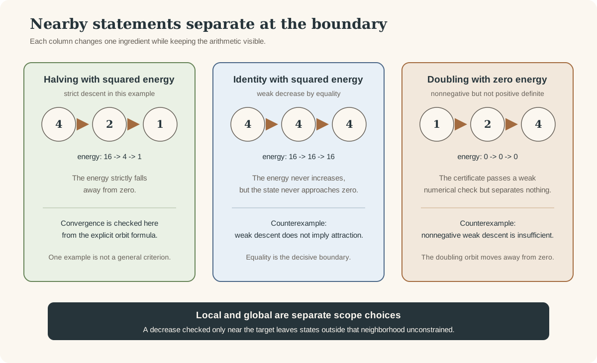
Strict descent alone is intentionally not an attraction theorem here. A strictly decreasing real sequence can approach a positive limit. Classical discrete LaSalle arguments add compact trapped trajectories and identify the largest invariant subset where the difference vanishes. Coercive or comparison-function arguments provide other routes. Those are later milestones, not invisible assumptions in this one.
Standalone Lean tutorial
The complete countdown-energy.lean file imports only Std. It proves the
finite countdown claims and the identity boundary. Run it on macOS or Linux:
elan run leanprover/lean4:v4.32.0 lean \
  site/content/knowledge-base/deep-dives/lyapunov-functions-and-the-direct-method-in-discrete-time/countdown-energy.lean
This standalone tutorial has a small resource profile. It does not import Mathlib and does not check the pseudo-metric direct-method theorem.
Try the full project interface
import NonlinearDynamics.Deterministic.Discrete.Lyapunov

#check IsPositiveDefiniteOn
#check IsWeakLyapunovDecreaseOn.antitone_orbit
#check HasSublevelControlAt
#check isAttractedTo_of_tendsto_lyapunov
NonlinearDynamics/Deterministic/Discrete/Lyapunov.lean; the full module check
uses the repository’s pinned Lean and Mathlib environment and may require
substantial disk space and setup time.cd formalization
lake env lean -DwarningAsError=true NonlinearDynamics/Deterministic/Discrete/Lyapunov.leanResource note: this exact file uses the repository's
pinned Lean and Mathlib dependencies. Initial project setup can require
substantial disk space and build time. For a lightweight first step on
macOS or Linux, use the page's standalone Lean-core or Std
tutorial.
Boundaries
This module proves no converse Lyapunov theorem, compact LaSalle invariance principle, exponential rate, invariant-set stability, periodic-orbit result, stable manifold, structural robustness, stochastic stability, ODE theorem, or Lyapunov-exponent statement. A decreasing certificate need not be physical energy, and scalar descent does not mean that every coordinate descends.
Continue with the shorter Lyapunov function glossary chapter or the declaration-complete Research Note.
References
- J. P. LaSalle, “Difference Equations. Discrete Semidynamical Systems,” sections 6, 7, and 10, in The Stability of Dynamical Systems, SIAM CBMS 25 (1976), pages 1–25, DOI 10.1137/1.9781611970432.ch1.
- Saber Elaydi, “Stability Theory,” Chapter 4 of An Introduction to Difference Equations, third edition, especially Theorems 4.20 and 4.24, DOI 10.1007/0-387-27602-5_4.
- James Hurt, “Some Stability Theorems for Ordinary Difference Equations,” SIAM Journal on Numerical Analysis 4(4), 582–596 (1967), DOI 10.1137/0704053.
- Mathlib 4.32.0, pinned revision
81a5d257, source modulesTopology.Order.LocalExtr,Data.Set.Function, andLogic.Function.Iterate.