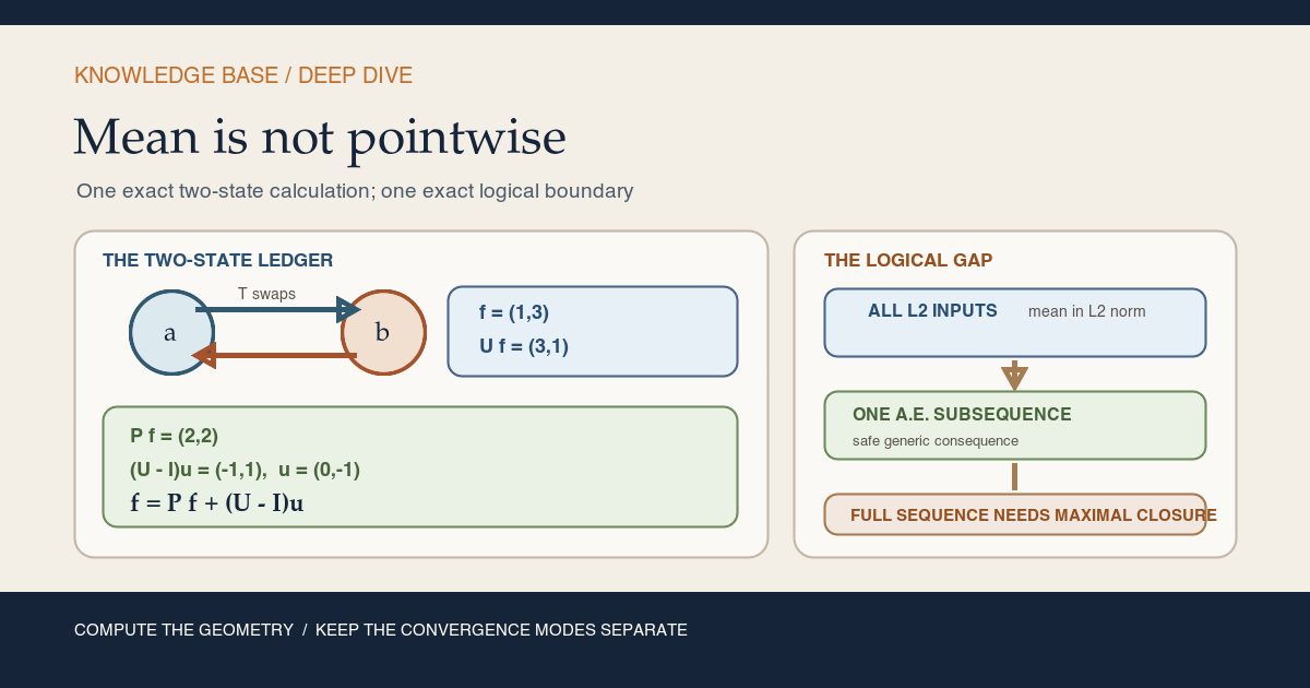
Base camp: calculate the complete two-state model
Begin with the probability space
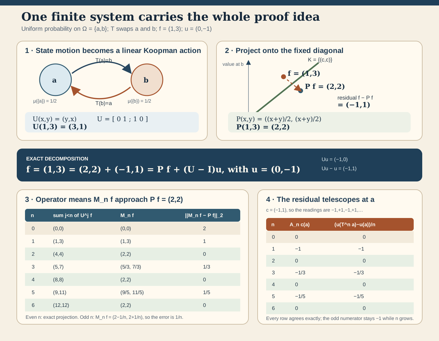
\[ \Omega=\{a,b\}, \qquad \mu(\{a\})=\mu(\{b\})=\frac12. \]The update \(T\) swaps the states:
\[ T(a)=b, \qquad T(b)=a. \]An observable is now just a pair
\[ f=(f(a),f(b)). \]Choose the real observable \(f=(1,3)\). One time step swaps its two readings, so the Koopman action is
\[ U_T(x,y)=(y,x), \qquad U_T= \begin{pmatrix} 0&1\\ 1&0 \end{pmatrix}, \qquad U_Tf=(3,1). \]The real \(L^2\) inner product remembers the probability weights:
\[ \langle(x,y),(r,s)\rangle_{L^2(\mu)} {} = \frac{xr+ys}{2}. \]A vector is fixed by \(U_T\) exactly when its two coordinates agree. Thus the fixed subspace and orthogonal projection are
\[ K=\{(c,c):c\in\mathbb R\}, \qquad P_K(x,y)= \left(\frac{x+y}{2},\frac{x+y}{2}\right). \]For the chosen observable,
\[ P_Kf=(2,2), \qquad f-P_Kf=(-1,1). \]The residual is not merely perpendicular to the fixed line. It is an exact forward coboundary. Take the simple potential \(u=(0,-1)\). Then
\[ U_Tu=(-1,0), \qquad (U_T-I)u=(-1,1)=f-P_Kf. \]So one finite calculation already exposes the decomposition used in the general proof:
\[ \boxed{f=(2,2)+(-1,1) =P_Kf+(U_T-I)u.} \]Compute the means approaching the projection
Let
\[ M_nf=\frac1n\sum_{j=0}^{n-1}U_T^jf \]for positive \(n\), and use Lean’s totalized value \(M_0f=(0,0)\). Direct calculation gives:
| Horizon \(n\) | Sum of the first \(n\) iterates | Mean \(M_nf\) | \(L^2(\mu)\) error from \((2,2)\) |
|---|---|---|---|
| 0 | \((0,0)\) | \((0,0)\) | \(2\) |
| 1 | \((1,3)\) | \((1,3)\) | \(1\) |
| 2 | \((4,4)\) | \((2,2)\) | \(0\) |
| 3 | \((5,7)\) | \((5/3,7/3)\) | \(1/3\) |
| 4 | \((8,8)\) | \((2,2)\) | \(0\) |
| 5 | \((9,11)\) | \((9/5,11/5)\) | \(1/5\) |
| 6 | \((12,12)\) | \((2,2)\) | \(0\) |
For \(n=2k\), the mean is exactly \((2,2)\). For \(n=2k+1\),
\[ M_nf=\left(2-\frac1n,2+\frac1n\right), \qquad \lVert M_nf-P_Kf\rVert_2=\frac1n. \]Both coordinates converge pointwise here because there are only two points. The general theorem proved by the module is deliberately weaker: it first asserts convergence in the \(L^2\) norm.
Compute the pointwise telescoping residual
At the start \(a\), the coboundary \(c=(-1,1)\) reads
\[ -1,\ +1,\ -1,\ +1,\ldots. \]Its average is zero at every positive even horizon and \(-1/n\) at every odd horizon. The endpoint formula explains those cancellations in one line:
\[ \frac1n\sum_{j=0}^{n-1}c(T^ja) {} = \frac{u(T^na)-u(a)}{n} {} = \begin{cases} 0,&n\text{ even},\\ -1/n,&n\text{ odd}. \end{cases} \]At \(b\), the odd value is \(+1/n\). In either case the full pointwise sequence tends to zero.
This example is finite, measurable, measure preserving, and a probability system. It is a genuine model of the formal theorem, not an analogy. It is also unusually friendly: norm and full pointwise convergence both hold by inspection. Later we will put beside it a different sequence whose \(L^2\) norm tends to zero while its full pointwise sequence fails to converge. That second sequence is a diagnostic for a logical implication, not a Birkhoff counterexample.
Four measure words will recur. A probability measure assigns total mass one; here the two singleton masses add to \(1/2+1/2=1\). A measure-preserving transformation does not change event masses under preimage; here swapping the two equal weights does nothing to them. A null set has measure zero. A statement holds almost everywhere when it may fail only on such a null set. On this two-point uniform space the only null set is the empty set, so “almost everywhere” actually means “at both \(a\) and \(b\).” On \([0,1)\), a nonempty singleton such as \(\{0\}\) is null, which is why the later typewriter subsequence may fail there and still converge almost everywhere.
A dynamical system moves states. Ergodic theory asks which information long orbit averages retain. Functional analysis changes the viewpoint: instead of following a state through time, it lets time act on every observable at once. The resulting composition operator is linear even when the state dynamics are nonlinear.
The power comes with a translation cost. A theorem about vectors in an \(L^2\) Hilbert space is a theorem about equivalence classes modulo null sets. A pointwise orbit average uses actual values at actual points. Moving from one world to the other requires representative bookkeeping, and moving from norm convergence to full-sequence almost-everywhere convergence requires a genuine stability theorem. Neither step is automatic.
Random-matrix-theory milestone 25 (RMT-25) formalizes the precise intermediate layer. It proves two results that should always be stated separately:
- for every real \(L^2\) observable, the Koopman operator averages converge in \(L^2\) norm to the orthogonal projection onto the fixed subspace; and
- fixed vectors plus coboundaries generated by \(L^2\) simple functions form a dense set whose chosen representatives have almost-everywhere convergent pointwise Birkhoff averages.
The declaration-complete implementation account is Koopman L² Mean Convergence and a Dense Pointwise-Good Core in Lean. The two recurring objects have compact entries at Koopman operator and Koopman coboundary . The orbit notation comes from the Birkhoff sum , and representative-level convergence is recorded by the Birkhoff convergence event .
Choose a route up
| Route | Begin | Destination |
|---|---|---|
| Intuition | Move states, pull observables | See why nonlinear dynamics produces a linear operator |
| Algebra | Coboundaries telescope | Reduce an entire orbit sum to two endpoints |
| Geometry | The fixed subspace is the summit target | Understand orthogonal projection and mean convergence |
| Density | Why simple coboundaries are enough | Build a dense pointwise-good core |
| Representatives | An L² equality is not a pointwise equality | Cross from quotient vectors to chosen functions safely |
| Convergence | The convergence ladder has a cliff | Separate norm, measure, subsequence, and full sequence |
| History | Four historical scopes, one modern specialization | Keep source lineage distinct from theorem identity |
| Lean | In Lean: seven bridges from the finite ledger to the checked theorem | Translate the human statement, paper mathematics, exact syntax, and commands |
| Practice | Solved exercises | Reconstruct every major bridge |
| Successor | What the later maximal-closure module adds | See how the next checked module closes the pointwise theorem |
Learning objectives
By the summit, a reader should be able to:
- distinguish forward state motion from observable pullback;
- define the Koopman operator \(U_Tf=f\circ T\);
- prove that measure preservation makes this operator an \(L^2\) isometry;
- explain why an isometry need not be a unitary equivalence;
- compute \(U_T^nf\) as \(f\circ T^n\);
- define the fixed subspace and its orthogonal projection;
- define the forward coboundary operator \(U_T-I\);
- telescope a forward coboundary average to two endpoint values;
- interpret the totalized horizon-zero identity without treating it as ordinary division by zero;
- derive pointwise convergence for a bounded coboundary potential;
- state the Hilbert-space mean-ergodic theorem used by RMT-25;
- explain why RMT-25 exposes only the operator bound \(\lVert U_T\rVert\le1\);
- decompose a vector into fixed and orthogonal parts;
- state the checked one-sided closure inclusion without upgrading it to equality;
- explain why continuous images of dense simple functions approximate arbitrary coboundaries;
- prove that fixed plus simple coboundary vectors form a dense set;
- distinguish an \(L^2\) vector from a chosen representative;
- explain the countable intersection used for a fixed representative;
- explain the finite-range representative used for a simple coboundary;
- state the almost-everywhere transport needed after composition and addition;
- follow norm convergence through convergence in measure to an almost-everywhere subsequence;
- explain why this ladder does not give full-sequence pointwise convergence;
- analyze the dyadic typewriter counterexample;
- distinguish the RMT-25 mean theorem from the RMT-25 dense-core theorem;
- audit every assumption that is absent from the public interface; and
- explain how a weak maximal estimate supplies the missing closure stability.
Move states, pull observables
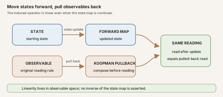
Let \((\Omega,\mu)\) be a measure space and let \(T:\Omega\to\Omega\) preserve \(\mu\). A state begins at \(\omega\), then moves through
\[ \omega,\quad T\omega,\quad T^2\omega,\quad \ldots. \]An observable \(f:\Omega\to\mathbb R\) assigns a number to each state. Rather than moving \(f\), one may ask what value the original observable reads after one state update. The Koopman operator is
\[ U_Tf=f\circ T, \qquad (U_Tf)(\omega)=f(T\omega). \]This direction matters. The state moves forward by \(T\), while the observable is pulled back by precomposition. The operator is linear:
\[ U_T(af+bg)=aU_Tf+bU_Tg. \]No linearity of \(T\) is required. Logistic maps, expanding maps, return maps, and nonlinear flows sampled at a fixed time all induce linear composition operators on suitable observable spaces.
Why measure preservation is the right analytic gate
The real \(L^2\) norm is
\[ \lVert f\rVert_2^2=\int_\Omega |f(\omega)|^2\,d\mu(\omega). \]If \(T\) preserves \(\mu\), integration after composition leaves this norm unchanged:
\[ \lVert U_Tf\rVert_2^2 {} = \int_\Omega |f(T\omega)|^2\,d\mu(\omega) {} = \int_\Omega |f(\omega)|^2\,d\mu(\omega). \]Thus \(U_T\) is a linear isometry on \(L^2\). RMT-25 packages it as a continuous linear map by taking Mathlib’s measure-preserving \(L^p\) composition isometry and forgetting only the bundled isometry structure (Mathlib \(L^p\) composition API).
An isometry need not be onto. A noninvertible measure-preserving map can still preserve every \(L^2\) norm, while its composition operator may fail to have an inverse. Therefore this module says Koopman isometry or Koopman contraction, not unitary equivalence. Invertibility is absent from every public theorem.
The project exposes
\[ \lVert U_T\rVert\le1 \]rather than unconditional equality. On the zero measure, every \(L^2\) vector is the zero equivalence class, so the operator norm is zero. For each vector, Mathlib’s underlying composition map still preserves its norm exactly. The public operator-norm inequality is the statement that remains correct without adding a nontriviality premise.
Iteration agrees in both worlds
Repeated composition gives
\[ U_T^n f=f\circ T^n. \]This identity is what lets a Birkhoff average of a Hilbert-space operator become the familiar orbit average of an observable:
\[ M_nf {} = \frac1n\sum_{j=0}^{n-1}U_T^j f. \]At the level of representatives, the \(j\)-th term reads \(f(T^j\omega)\). At the level of \(L^2\), the entire sum is a vector. RMT-25 keeps these readings related but not conflated.
Coboundaries telescope
Take any real-valued potential \(u\). Its forward coboundary is
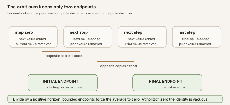
\[ d=U_Tu-u, \qquad d(\omega)=u(T\omega)-u(\omega). \]The sign convention is \(U_T-I\). Some texts use \(I-U_T\); every cancellation then has the opposite sign, but the range and convergence ideas are the same. RMT-25 fixes one convention so later proofs cannot silently switch.
The first \(n\) terms telescope:
\[ \begin{aligned} \sum_{j=0}^{n-1}d(T^j\omega) &=\sum_{j=0}^{n-1} \left(u(T^{j+1}\omega)-u(T^j\omega)\right)\\ &=u(T^n\omega)-u(\omega). \end{aligned} \]Therefore the average is exactly
\[ A_nd(\omega) {} = n^{-1}\left(u(T^n\omega)-u(\omega)\right). \]Lean’s inverse is totalized. At \(n=0\), the left side is an empty average and the right side is \(0^{-1}\) times a zero endpoint difference, so both sides are zero. The equality is valid there, but it carries no positive-time averaging information.
If the range of \(u\) is bounded, there is a constant \(C\) with
\[ |u(T^n\omega)-u(\omega)|\le C \]for every \(\omega\) and \(n\). Hence
\[ |A_nd(\omega)|\le \frac{C}{n}\longrightarrow0. \]This result is pointwise and raw. It uses no measurable space, no measure, no integrability, and no invariance. Global boundedness is a convenient sufficient condition. Along one orbit, boundedness of the orbit values would suffice; sublinear endpoint growth would suffice as well. RMT-25 states the reusable globally bounded version.
Constant potentials give the zero coboundary. Identity dynamics also give the zero coboundary operator on every \(L^2\) vector. These are compiled probes, not assumptions.
The fixed subspace is the summit target
Define
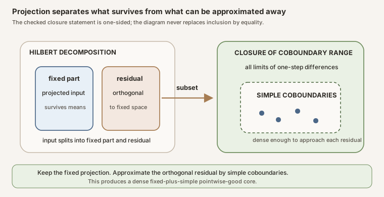
\[ K=\operatorname{Fix}(U_T) {} = \{f\in L^2:U_Tf=f\}. \]This is a closed real subspace. Because \(L^2\) is a complete Hilbert space, every vector \(f\) has an orthogonal decomposition
\[ f=P_Kf+r, \qquad P_Kf\in K, \qquad r\in K^\perp. \]The map \(P_K\) is the orthogonal projection onto the fixed subspace. Its geometric meaning is direct: the part \(P_Kf\) survives averaging, while the orthogonal remainder is washed out in norm (Mathlib orthogonal projection).
Mathlib’s Hilbert-space mean-ergodic theorem says that if \(L\) is a continuous linear map on a complete real or complex Hilbert space and \(\lVert L\rVert\le1\), then
\[ \frac1n\sum_{j=0}^{n-1}L^jf \longrightarrow P_{\operatorname{Fix}(L)}f \]in norm. RMT-25 specializes this theorem to \(L=U_T\):
\[ M_nf\longrightarrow P_Kf \quad\text{in }L^2. \]The result assumes only measure preservation. It does not require finite total mass, probability normalization, sigma-finiteness as a separate premise, ergodicity, injectivity, surjectivity, or invertibility.
What ergodicity would change, but does not enter here
On an ergodic probability space, the fixed subspace is often identified with the constants, and the projection can then be identified with the integral of the observable. RMT-25 proves neither identification. Its target is the abstract fixed-space projection. That form is valid before probability or ergodicity is available, and it avoids silently turning an invariant function into a constant.
Why the exponent two matters here
The statement uses \(L^2\) because orthogonal complements and orthogonal projections are Hilbert-space tools. This does not mean no mean theorem exists outside \(L^2\). It means this proof route, and this precise projection API, uses inner-product geometry. The successor pointwise theorem lives naturally in \(L^1\) and uses a different stability mechanism.
Coboundaries fill the orthogonal directions
Let
\[ C=U_T-I. \]The checked Hilbert argument proves the one-sided inclusion
\[ K^\perp \subseteq \overline{\operatorname{range}(C)}. \]The direction and the closure both matter. The public declaration does not state equality. A figure or summary that replaces the inclusion sign by an equality would claim more than this module exports.
The proof takes orthogonal complements. If a vector \(x\) is orthogonal to the range of \(C\), then
\[ \langle (U_T-I)y,x\rangle=0 \quad\text{for every }y, \]so
\[ \langle U_Ty,x\rangle=\langle y,x\rangle. \]The contraction estimate and the Hilbert equality case force \(x\) to be fixed. Taking the orthogonal complement again and using the double-orthogonal closure theorem yields the displayed inclusion.
Why simple coboundaries are enough
An arbitrary \(L^2\) generator for a coboundary need not have a bounded chosen representative. Simple functions solve both the approximation problem and the pointwise problem.
A simple function takes only finitely many values. Its range is therefore bounded. Mathlib proves that \(L^p\) simple functions are dense whenever the exponent is not infinity; no finite-measure or sigma-finite assumption is needed for the \(p=2\) use here.
The coboundary operator \(C\) is continuous. A continuous map sends an approximating sequence of simple vectors to an approximating sequence of simple-generated coboundaries. Consequently,
\[ K^\perp \subseteq \overline{C(\text{simple }L^2\text{ vectors})}. \]Now decompose any \(f\in L^2\) as \(f=p+r\), where \(p=P_Kf\in K\) and \(r\in K^\perp\). Approximate \(r\) by simple-generated coboundaries \(c_m\). Then
\[ p+c_m\longrightarrow p+r=f. \]This proves density of the set
\[ \mathcal G {} = \{p+c:p\in K, c=C(u), u\text{ is an }L^2\text{ simple vector}\}. \]RMT-25 exports \(\mathcal G\) as a set and proves it dense. It does not package that set as a submodule. Density is the property needed for the later closure argument.
An L² equality is not a pointwise equality
The Hilbert space \(L^2(\mu)\) identifies functions that agree almost everywhere. A vector \(f\in L^2\) is not one raw function together with a proof that all equalities hold pointwise. Lean therefore forces the representative bridge to be explicit.
This is not bureaucratic friction. If one changes a representative on a null set, then every orbit that later enters that set may see changed pointwise values. Measure preservation controls the preimages of those null sets, which is why it is the exact bridge hypothesis.
Fixed vectors: intersect all iterate equalities
Suppose \(h\in K\), so \(U_Th=h\) in \(L^2\). Iterating gives
\[ U_T^nh=h \quad\text{in }L^2 \]for every natural \(n\). Mathlib’s composition representative theorem converts each equality into
\[ h(T^n\omega)=h(\omega) \quad\text{for almost every }\omega. \]The exceptional set can depend on \(n\). Because the natural numbers are countable, RMT-25 intersects the conull sets for all \(n\). On the resulting single conull set, the entire orbit is constant under the chosen representative. Every positive-time Birkhoff average then equals \(h(\omega)\), so the sequence converges.
Skipping the countable intersection would prove only a family of almost-everywhere equalities, not one orbitwise statement valid at all times.
Simple coboundaries: choose a finite-range representative
Let \(u\) be an \(L^2\) simple vector. Mathlib supplies a raw simple function \(v:\Omega\to\mathbb R\) such that
\[ v=u \quad\text{almost everywhere}. \]Its finite range is bounded. Measure preservation is in particular quasi-measure-preserving, so the equality transports through \(T\):
\[ v\circ T=u\circ T \quad\text{almost everywhere}. \]The chosen representative of \(Cu=U_Tu-u\) is therefore almost everywhere equal to the raw bounded coboundary
\[ v\circ T-v. \]The raw telescope proves pointwise convergence to zero for every starting point. The RMT-22 representative transport theorem then transfers membership in the Birkhoff convergence event back to the chosen \(L^2\) representative.
Sums: transport once more
The sum of two convergent real sequences converges. RMT-25 proves a private raw closure lemma for the Birkhoff convergence event under addition. It combines the fixed representative and simple-coboundary representative results, then uses Mathlib’s almost-everywhere representative equality for \(h+c\) and the RMT-22 event transport one final time.
The conclusion is
\[ f\in\mathcal G \quad\Longrightarrow\quad \text{the chosen representative of }f\text{ has convergent Birkhoff averages almost everywhere}. \]The theorem asserts existence of a pointwise limit. It does not identify that limit with \(P_Kf\). For the fixed-plus-coboundary core such an identification is mathematically expected from the construction, but it is not the exported representative theorem and should not be attributed to it.
The convergence ladder has a cliff
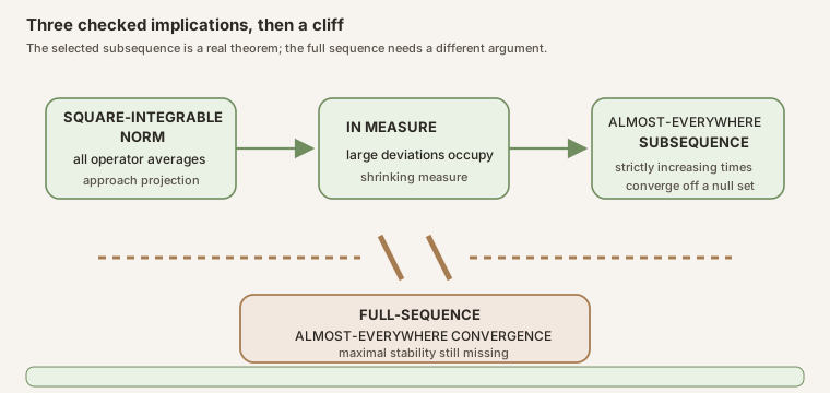
The mean theorem gives
\[ M_nf\longrightarrow P_Kf \quad\text{in }L^2. \]Mathlib formalizes the safe ladder:
\[ L^2\text{ norm convergence} \Longrightarrow \text{convergence in measure} \Longrightarrow \text{an almost-everywhere convergent subsequence}. \]The two formal bridges are Mathlib’s norm-to-measure and measure-to-almost-everywhere-subsequence theorems (Mathlib convergence in measure).
RMT-25 exports the specialized subsequence theorem. There exists a strictly increasing map \(n_s:\mathbb N\to\mathbb N\) such that the chosen representatives of \(M_{n_s(i)}f\) converge almost everywhere to the chosen representative of \(P_Kf\).
Nothing in that chain upgrades the selected subsequence to the entire sequence.
The dyadic typewriter warning
On \([0,1)\) with Lebesgue probability measure, enumerate the half-open dyadic intervals level by level. Give the interval in position \(k\) at level \(m\) the global index
\[ n=2^m+k, \qquad 0\le k\lt2^m, \]and define
\[ q_{2^m+k} {} = \mathbf 1_{[k/2^m,(k+1)/2^m)}. \]The first levels are
\[ [0,1), \quad [0,\tfrac12),[\tfrac12,1), \quad [0,\tfrac14),[\tfrac14,\tfrac12),[\tfrac12,\tfrac34),[\tfrac34,1), \quad\ldots \]At level \(m\), each interval has length \(2^{-m}\), so
\[ \lVert q_n\rVert_2^2=2^{-m}\longrightarrow0. \]Thus \(q_n\to0\) in \(L^2\). Now pin down one point rather than saying “typically.” At \(x=5/8\), the containing cell has positions
\[ k=0,1,2,5,10,\ldots \]at levels \(m=0,1,2,3,4,\ldots\). Therefore the value one occurs at global indices
\[ n=1,3,6,13,26,\ldots. \]There are zeros between those hits. The sequence \(q_n(5/8)\) therefore has infinitely many zeros and infinitely many ones, so it does not converge. Indeed every \(x\in[0,1)\) belongs to exactly one interval at every level, and the same obstruction holds at every point.
The subsequence issue is different. Select the leftmost interval at each level:
\[ q_{2^m}=\mathbf 1_{[0,2^{-m})}. \]For every \(x\gt0\), this selected subsequence is eventually zero. At \(x=0\) it is always one. The exceptional singleton \(\{0\}\) has Lebesgue measure zero, so this subsequence converges to zero almost everywhere. One sequence therefore exhibits both facts:
\[ q_n\to0\text{ in }L^2, \qquad q_{2^m}\to0\text{ a.e.}, \qquad q_n(x)\text{ fails to converge for the full sequence}. \]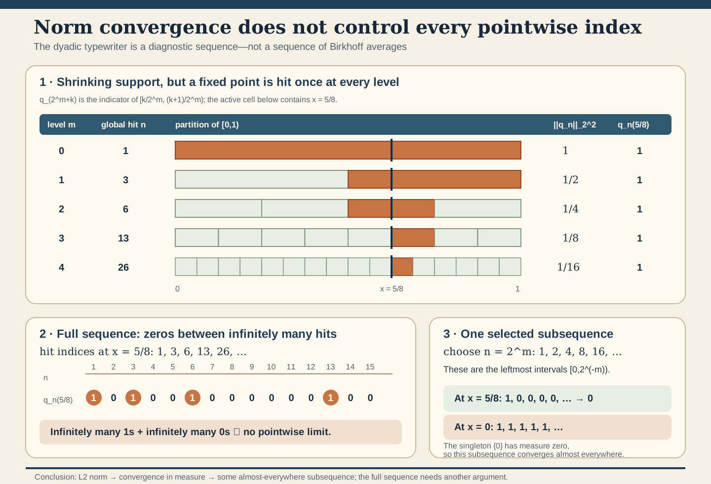
Two achievements that density does not merge
It is tempting to argue:
- all \(L^2\) averages converge in norm;
- a dense set has pointwise-convergent averages;
- therefore every \(L^2\) vector has pointwise-convergent averages.
Step 3 is invalid without continuity of the pointwise-good property in the \(L^2\) or \(L^1\) topology. Pointwise convergence is not a norm-closed property for arbitrary sequences of operators. Density tells us that every target can be approximated by good inputs. A maximal inequality is needed to control the orbit-average error uniformly over all times.
The two RMT-25 routes should therefore remain visibly parallel:
\[ \text{all }L^2\text{ inputs} \longrightarrow \text{norm convergence}, \]\[ \text{dense special inputs} \longrightarrow \text{full-sequence pointwise convergence almost everywhere}. \]Neither route contains the other.
Exact assumption ledger
| Layer | Assumptions used | Assumptions not used |
|---|---|---|
| Endpoint coboundary identity | A type, a self-map, a real potential, a natural horizon | Measurability, measure, boundedness |
| Bounded-coboundary pointwise limit | Bounded range of the potential | Measurability, measure, preservation |
| Koopman operator and iterate formula | MeasurePreserving T μ μ | Finite mass, probability, ergodicity, inverse |
| Hilbert mean convergence | Measure preservation plus real \(L^2\) Hilbert structure | Sigma-finiteness as a separate premise, injectivity, surjectivity |
| Simple-coboundary density | The same preservation interface and \(p=2\ne\infty\) | Finite total mass, probability |
| Representative bridge | Measure preservation, which supplies quasi-measure preservation | Ergodicity, invertibility, a selected pointwise limit formula |
| Subsequence theorem | The checked \(L^2\) norm limit | A full-sequence almost-everywhere conclusion |
The translation \(z\mapsto z+1\) on integer counting measure is a compiled
infinite-measure probe. The dense-core and pointwise-good theorems apply even
though this is not a probability space. A constant map on Bool preserves a
Dirac measure while failing injectivity; the final theorem applies there too.
These probes show that the absent assumptions are truly absent from the API.
Four historical scopes, one modern specialization
RMT-25 is a modern specialization assembled from current Mathlib interfaces. It is not a line-by-line formalization of any one historical paper.
| Source | Setting and result | Relationship to RMT-25 |
|---|---|---|
| Koopman 1931 | Continuous-time Hamiltonian flow, invariant positive density, complex Hilbert space, one-parameter unitary group \(U_tf=f\circ S_t\) | Historical composition-operator construction; RMT-25 is discrete, real, and permits noninvertible maps |
| von Neumann 1932 | Continuous-time unitary dynamics; interval averages converge strongly, meaning in Hilbert norm, to a spectral fixed-space projection | Historical mean theorem; RMT-25 uses Mathlib’s discrete contraction theorem rather than von Neumann’s spectral proof |
| Birkhoff 1931 | Pointwise occupation-time theorem for volume-preserving flows, explicitly contrasted with convergence in the mean | Historical pointwise counterpart; not the exact modern discrete \(L^1\) API proved here |
| Keane and Petersen 2006 | Probability space, possibly noninvertible measure-preserving map, \(L^1\) observable, maximal-to-pointwise proof | Closest roadmap precedent for the later maximal-closure module, not the source of RMT-25’s Hilbert geometry |
On page 71, von Neumann defines strong convergence as Hilbert-norm convergence. Pages 72–74 prove interval-average convergence to the spectral projection. His pages 77–78 include an almost-everywhere subsequence statement, not a general full-sequence pointwise theorem. Birkhoff opens his paper by contrasting the convergence-in-mean result with the pointwise problem. Those primary-source distinctions are why this chapter does not use mean and pointwise as synonyms.
The DOI for Birkhoff’s article is the historically odd
10.1073/pnas.17.2.656, even though the bibliographic issue is 17(12). The
reference below preserves the DOI assigned by the journal record.
The formal architecture
The checked RMT-25 Lean module follows four layers.
Layer 1: raw orbit algebra
birkhoffAverage_forwardCoboundary proves the exact endpoint formula, including
the totalized zero horizon. tendsto_birkhoffAverage_forwardCoboundary obtains
the bounded-potential pointwise limit.
Layer 2: Koopman Hilbert geometry
The module defines koopmanL2, koopmanFixedSubspaceL2,
koopmanInvariantProjectionL2, koopmanCoboundaryL2, the simple-coboundary
set, and the fixed-plus-simple set. It proves application, iteration, and the
operator-norm bound.
A private contraction lemma converts orthogonality to the range of \(U-I\)
into fixedness. The public theorem states
fixedOrthogonal_le_closure_range_koopmanL2 through the named coboundary
operator. Simple-function density and projection decomposition then prove
dense_fixedPlusSimpleCoboundarySetL2.
Layer 3: convergence modes
tendsto_birkhoffAverage_koopmanL2 and its project-named projection variant
state the \(L^2\) norm theorem. The deliberately explicit
exists_subsequence_ae_tendsto_birkhoffAverage_koopmanL2_projection records the
strongest generic representative consequence used here: one strictly
increasing almost-everywhere convergent subsequence.
Layer 4: the pointwise-good core
Separate theorems handle fixed representatives and simple coboundaries. A private addition lemma closes the raw convergence event under sums. The final theorem states almost-everywhere event membership for every vector in the dense fixed-plus-simple core.
The module ends with eleven documented compiled probes and five #print axioms
checks. The printed footprint is exactly propext, Classical.choice, and
Quot.sound; there is no project axiom or proof hole.
In Lean: seven bridges from the finite ledger to the checked theorem
The two-state ledger used ordinary pairs so that every number remained visible. The project module works with real \(L^2\) equivalence classes and measure-preserving maps. These seven bridges show exactly where each elementary idea appears in the general interface.
Bridge 1: pull an observable back through the state update
koopmanL2_apply hT fhT : MeasurePreserving T μ μcertifies that the update preserves the same measure.f : Lp ℝ 2 μis a real square-integrable equivalence class.koopmanL2 hT fis the project operator application.- The theorem rewrites it to Mathlib’s
Lp.compMeasurePreserving T hT f. At the chosen-representative level, Mathlib later supplies the almost-everywhere equation with \(f\circ T\). - The iterate companion is
iterate_koopmanL2_apply hT n f; it identifies \(U_T^nf\) with composition by \(T^n\).
Bridge 2: name the fixed line and its orthogonal projection
koopmanInvariantProjectionL2 hT fkoopmanFixedSubspaceL2 hTis built witheqLocus, the subspace wherekoopmanL2 hTand the identity operator agree.koopmanInvariantProjectionL2 hTis that subspace’s bundledstarProjection.- In the two-state example,
eqLocusis the diagonal \(\{(c,c)\}\), and the displayed Lean term evaluates mathematically to \((2,2)\) when \(f=(1,3)\). - The project theorem does not identify this projection with a conditional expectation or with a constant. Those require additional checked structure.
Bridge 3: telescope a forward coboundary exactly
birkhoffAverage_forwardCoboundary u n ωbirkhoffAverage ℝ Tis Mathlib’s real, totalized finite orbit average.fun x ↦ u (T x) - u xfixes the sign convention \(U_T-I\).T^[n] ωis Lean’s \(n\)-fold iterate \(T^n\omega\).(n : ℝ)⁻¹ •means scalar multiplication by the reciprocal of the real number corresponding ton.- No measurable space or measure is used. The companion
tendsto_birkhoffAverage_forwardCoboundaryadds only boundedness of the range ofuand concludes pointwise convergence to zero.
Bridge 4: make the fixed-plus-simple core dense
dense_fixedPlusSimpleCoboundarySetL2 hTsimpleKoopmanCoboundarySetL2 hTis the image of Mathlib’s dense setLp.simpleFunc ℝ 2 μunder \(U_T-I\).fixedPlusSimpleCoboundarySetL2 hTrecords sums \(h+c\), with \(h\) fixed and \(c\) in that image.- The geometric input
fixedOrthogonal_le_closure_range_koopmanL2 hTis one-sided: \(K^\perp\) lies in the closed coboundary range. It does not state equality. - Continuity of the coboundary operator transfers simple-function density, and the projection decomposition \(f=P_Kf+(f-P_Kf)\) finishes the proof.
Bridge 5: state mean convergence in the correct topology
tendsto_birkhoffAverage_koopmanL2_projection hT fbirkhoffAverage ℝ (koopmanL2 hT) id n faverages the vectors \(f,U_Tf,\ldots,U_T^{n-1}f\).Tendsto … atTop (nhds …)expresses convergence as the natural horizon tends to infinity in the norm topology of \(L^2\).norm_koopmanL2_le hTsupplies the contraction premise \(\lVert U_T\rVert\le1\) required by Mathlib’s Hilbert-space mean theorem.- Nothing in this declaration evaluates a chosen representative at one outcome, and nothing says that the full pointwise sequence converges.
Bridge 6: extract exactly one almost-everywhere subsequence
exists_subsequence_ae_tendsto_birkhoffAverage_koopmanL2_projection hT f∃ ns : ℕ → ℕ, StrictMono nschooses the subsequence indices.∀ᵐ ω ∂μmeans “for almost every \(\omega\) with respect to \(\mu\).”- Inside that conull set,
Tendsto … atTop (nhds …)is ordinary real convergence of the selected representative values. - The proof goes from \(L^2\) norm convergence to convergence in measure and
then invokes an almost-everywhere subsequence theorem. The quantifier is
about
ns i, not every natural horizon. The typewriter ledger shows why that distinction cannot be erased.
Bridge 7: prove full-sequence pointwise convergence on the dense core
ae_mem_birkhoffConvergenceSet_of_mem_fixedPlusSimpleCoboundarySetL2 hT hfhf : f ∈ fixedPlusSimpleCoboundarySetL2 hTsupplies the decomposition \(f=h+c\).birkhoffConvergenceSet T (fun ω ↦ f ω)is the set where the full natural-indexed average sequence tends to some finite real value.- The fixed part uses one countable intersection so every iterate-level representative equality holds at the same outcome.
- The simple part chooses a finite-range representative, applies the raw bounded telescope, and transports the event across almost-everywhere equality.
- This theorem is full-sequence but only for the dense core. Bridge 6 is for every \(L^2\) vector but only for one subsequence. RMT-25 never merges those quantifiers.
Try the exact declarations in the repository
The authoritative source is
formalization/NonlinearDynamics/Random/RandomCocycles/KoopmanL2Mean.lean.
For a full project check, save the following temporary query file as
formalization/NonlinearDynamics/KoopmanL2MeanChecks.lean:
import NonlinearDynamics.Random.RandomCocycles.KoopmanL2Mean

open MeasureTheory Set Filter Function
open NonlinearDynamics.Random.RandomCocycles

#check birkhoffAverage_forwardCoboundary
#check tendsto_birkhoffAverage_forwardCoboundary
#check koopmanL2
#check koopmanFixedSubspaceL2
#check koopmanInvariantProjectionL2
#check koopmanCoboundaryL2
#check simpleKoopmanCoboundarySetL2
#check fixedPlusSimpleCoboundarySetL2
#check koopmanL2_apply
#check iterate_koopmanL2_apply
#check norm_koopmanL2_le
#check fixedOrthogonal_le_closure_range_koopmanL2
#check fixedOrthogonal_subset_closure_simpleKoopmanCoboundarySetL2
#check dense_fixedPlusSimpleCoboundarySetL2
#check tendsto_birkhoffAverage_koopmanL2
#check tendsto_birkhoffAverage_koopmanL2_projection
#check exists_subsequence_ae_tendsto_birkhoffAverage_koopmanL2_projection
#check ae_mem_birkhoffConvergenceSet_of_mem_koopmanFixedSubspaceL2
#check ae_mem_birkhoffConvergenceSet_of_mem_simpleKoopmanCoboundarySetL2
#check ae_mem_birkhoffConvergenceSet_of_mem_fixedPlusSimpleCoboundarySetL2
Then type:
cd formalization
lake env lean NonlinearDynamics/KoopmanL2MeanChecks.lean
The twenty checks follow the public declarations in source order. Delete the temporary query file after the check. To compile the authoritative module itself, type:
cd formalization
lake env lean NonlinearDynamics/Random/RandomCocycles/KoopmanL2Mean.lean
Both commands import the pinned Mathlib graph and may require substantial disk space and memory.
cd formalization
lake env lean -DwarningAsError=true NonlinearDynamics/Random/RandomCocycles/KoopmanL2Mean.lean
Resource note: this exact file uses the repository's
pinned Lean and Mathlib dependencies. Initial project setup can require
substantial disk space and build time. For a lightweight first step on
macOS or Linux, use the page's standalone Lean-core or Std
tutorial.
Type the two-state and typewriter ledgers yourself with Lean and Std
This worksheet uses exact rational arithmetic. It computes the two-state Koopman action, fixed projection, coboundary, horizons zero through six, and the pointwise endpoint quotient. It then computes the typewriter values at \(x=5/8\), the hit indices \(1,3,6,13,26\), the exact squared norms, and the leftmost subsequence at an ordinary point and at its one exceptional endpoint.
It is a pedagogical finite model, not the project \(L^2\) proof. It imports no
Mathlib, defines no measure, and asserts no infinite limit. Save this exact
text as /tmp/KoopmanL2MeanTutorial.lean:
import Std

namespace KoopmanL2MeanTutorial

structure Vec2 where
  a : Rat
  b : Rat
  deriving Repr, DecidableEq

def zero : Vec2 := ⟨0, 0⟩

def add (v w : Vec2) : Vec2 := ⟨v.a + w.a, v.b + w.b⟩

def sub (v w : Vec2) : Vec2 := ⟨v.a - w.a, v.b - w.b⟩

def scale (r : Rat) (v : Vec2) : Vec2 := ⟨r * v.a, r * v.b⟩

def koopman (v : Vec2) : Vec2 := ⟨v.b, v.a⟩

def projection (v : Vec2) : Vec2 :=
  let mean := (v.a + v.b) / 2
  ⟨mean, mean⟩

def iterateKoopman : Nat → Vec2 → Vec2
  | 0, v => v
  | n + 1, v => iterateKoopman n (koopman v)

def sumIterates : Nat → Vec2 → Vec2
  | 0, _ => zero
  | n + 1, v => add (sumIterates n v) (iterateKoopman n v)

def meanAverage (n : Nat) (v : Vec2) : Vec2 :=
  if n = 0 then zero else scale (1 / (n : Rat)) (sumIterates n v)

inductive Point where
  | a
  | b
  deriving Repr, DecidableEq

def step : Point → Point
  | .a => .b
  | .b => .a

def iteratePoint : Nat → Point → Point
  | 0, p => p
  | n + 1, p => iteratePoint n (step p)

def value (v : Vec2) : Point → Rat
  | .a => v.a
  | .b => v.b

def orbitAverage (v : Vec2) (n : Nat) (p : Point) : Rat :=
  value (meanAverage n v) p

def telescope (u : Vec2) (n : Nat) (p : Point) : Rat :=
  if n = 0 then 0
  else (value u (iteratePoint n p) - value u p) / (n : Rat)

def twoPow (m : Nat) : Nat := 2 ^ m

def hitAtLevel (m k xNum xDen : Nat) : Bool :=
  let scaledX := xNum * twoPow m
  k * xDen ≤ scaledX && scaledX < (k + 1) * xDen

def levelRow (m xNum xDen : Nat) : List Bool :=
  (List.range (twoPow m)).map fun k => hitAtLevel m k xNum xDen

def typewriterPrefix (levels xNum xDen : Nat) : List Bool :=
  (List.range levels).flatMap fun m => levelRow m xNum xDen

def hitIndices (levels xNum xDen : Nat) : List Nat :=
  ((typewriterPrefix levels xNum xDen).zip
      (List.range (twoPow levels - 1))).filterMap fun
    | (true, i) => some (i + 1)
    | (false, _) => none

def squaredNorms (levels : Nat) : List Rat :=
  (List.range levels).map fun m => 1 / (twoPow m : Rat)

def f : Vec2 := ⟨1, 3⟩
def u : Vec2 := ⟨0, -1⟩
def c : Vec2 := sub (koopman u) u

#eval koopman f
#eval projection f
#eval sub f (projection f)
#eval c
#eval (List.range 7).map fun n => (n, meanAverage n f)
#eval (List.range 7).map fun n =>
  (n, orbitAverage c n .a, telescope u n .a)
#eval typewriterPrefix 4 5 8
#eval hitIndices 5 5 8
#eval squaredNorms 5
#eval (List.range 5).map fun m => hitAtLevel m 0 5 8
#eval (List.range 5).map fun m => hitAtLevel m 0 0 1

example : koopman f = ⟨3, 1⟩ := by native_decide
example : projection f = ⟨2, 2⟩ := by native_decide
example : c = sub f (projection f) := by native_decide
example :
    (List.range 7).map (fun n => meanAverage n f) =
      [⟨0, 0⟩, ⟨1, 3⟩, ⟨2, 2⟩, ⟨5 / 3, 7 / 3⟩,
        ⟨2, 2⟩, ⟨9 / 5, 11 / 5⟩, ⟨2, 2⟩] := by
  native_decide
example :
    (List.range 20).all (fun n =>
      orbitAverage c n .a = telescope u n .a) = true := by
  native_decide
example : hitIndices 5 5 8 = [1, 3, 6, 13, 26] := by
  native_decide

end KoopmanL2MeanTutorial
From any directory, type:
source "$HOME/.elan/env"
elan run leanprover/lean4:v4.32.0 lean \
  /tmp/KoopmanL2MeanTutorial.lean
The byte-for-byte standard output emitted by Lean is:
{ a := 3, b := 1 }
{ a := 2, b := 2 }
{ a := -1, b := 1 }
{ a := -1, b := 1 }
[(0, { a := 0, b := 0 }),
 (1, { a := 1, b := 3 }),
 (2, { a := 2, b := 2 }),
 (3, { a := (5 : Rat)/3, b := (7 : Rat)/3 }),
 (4, { a := 2, b := 2 }),
 (5, { a := (9 : Rat)/5, b := (11 : Rat)/5 }),
 (6, { a := 2, b := 2 })]
[(0, 0, 0),
 (1, -1, -1),
 (2, 0, 0),
 (3, (-1 : Rat)/3, (-1 : Rat)/3),
 (4, 0, 0),
 (5, (-1 : Rat)/5, (-1 : Rat)/5),
 (6, 0, 0)]
[true, false, true, false, false, true, false, false, false, false, false, false, true, false, false]
[1, 3, 6, 13, 26]
[1, (1 : Rat)/2, (1 : Rat)/4, (1 : Rat)/8, (1 : Rat)/16]
[true, false, false, false, false]
[true, true, true, true, true]
The first four lines are \(U_Tf\), \(P_Kf\), the projection residual, and the
coboundary. The two tuple ledgers reproduce the tables above. In the
typewriter output, true means “the point lies in this interval.”
The final two lines say that \(5/8\) leaves the leftmost intervals after level
zero, while \(0\) never leaves them.
Standalone tutorial, suitable for a normal macOS or Linux machine. It
imports only Std and never opens the project’s Mathlib dependency
graph. This exact file and Lean output were checked with the pinned Lean 4.32.0
toolchain. The exact project declarations use the full project commands in the
preceding repository box.
Complete source-order declaration and helper map
The checked module is 491 lines and has SHA-256
4041dd4fcbb1353c31fa26072071c2e6ee73626eb5c8b7f59ac4d76219e446ac.
It contains twenty public declarations, two named private helpers, eleven
anonymous compiled boundary probes, and five axiom-footprint queries.
| Source order | Visibility | Declaration or helper | Exact role |
|---|---|---|---|
| 1 | public | birkhoffAverage_forwardCoboundary | Exact totalized endpoint identity for the raw forward coboundary |
| 2 | public | tendsto_birkhoffAverage_forwardCoboundary | Bounded potential gives pointwise convergence of those averages to zero |
| A | private | fixedOrthogonal_le_closure_range_sub_one | General contraction lemma placing the fixed orthogonal complement in the closed range of \(L-I\) |
| 3 | public | koopmanL2 | Real \(L^2\) measure-preserving composition as a continuous linear map |
| 4 | public | koopmanFixedSubspaceL2 | Equalizer of the Koopman and identity operators |
| 5 | public | koopmanInvariantProjectionL2 | Orthogonal projection onto that fixed subspace |
| 6 | public | koopmanCoboundaryL2 | The forward coboundary operator \(U_T-I\) |
| 7 | public | simpleKoopmanCoboundarySetL2 | Coboundaries generated by Mathlib \(L^2\) simple vectors |
| 8 | public | fixedPlusSimpleCoboundarySetL2 | Sums of fixed vectors and simple-generated coboundaries |
| 9 | public | koopmanL2_apply | Rewrites project application to Mathlib measure-preserving composition |
| 10 | public | iterate_koopmanL2_apply | Identifies \(U_T^nf\) with composition by \(T^n\) |
| 11 | public | norm_koopmanL2_le | Proves the unconditional operator bound \(\lVert U_T\rVert\le1\) |
| 12 | public | fixedOrthogonal_le_closure_range_koopmanL2 | Specializes private helper A to the named Koopman coboundary |
| 13 | public | fixedOrthogonal_subset_closure_simpleKoopmanCoboundarySetL2 | Replaces arbitrary generators by dense simple generators |
| 14 | public | dense_fixedPlusSimpleCoboundarySetL2 | Proves the fixed-plus-simple set dense in real \(L^2\) |
| 15 | public | tendsto_birkhoffAverage_koopmanL2 | Mean theorem with Mathlib’s orthogonal-projection target |
| 16 | public | tendsto_birkhoffAverage_koopmanL2_projection | Same norm theorem with the project’s projection name |
| 17 | public | exists_subsequence_ae_tendsto_birkhoffAverage_koopmanL2_projection | Extracts one strictly increasing almost-everywhere convergent subsequence |
| 18 | public | ae_mem_birkhoffConvergenceSet_of_mem_koopmanFixedSubspaceL2 | Gives full-sequence convergence almost everywhere for fixed representatives |
| 19 | public | ae_mem_birkhoffConvergenceSet_of_mem_simpleKoopmanCoboundarySetL2 | Gives full-sequence convergence almost everywhere for simple coboundaries |
| B | private | mem_birkhoffConvergenceSet_add | Adds two raw pointwise convergence witnesses |
| 20 | public | ae_mem_birkhoffConvergenceSet_of_mem_fixedPlusSimpleCoboundarySetL2 | Combines the two core pieces and transports the chosen sum representative |
Private helper A uses the contraction bound, Hilbert equality case, and the double-orthogonal closure identity. Private helper B uses finite-average linearity and addition of limits. Because they are private, they cannot be queried from the external scratch import; the table maps them where they actually occur in the source.
The eleven probes exercise: horizon zero; a constant potential; identity
Koopman, coboundary, projection, and representative behavior; the zero-measure
operator norm; the generic subsequence boundary; infinite counting measure; a
noninjective Dirac-preserving map; and the finite-range representative of a
simple vector. The five #print axioms commands sample one raw
limit, density, mean convergence, subsequence convergence, and the final core
theorem. Their checked footprint is exactly propext,
Classical.choice, and Quot.sound.
Additional boundary microexamples
Identity dynamics
If \(T=\mathrm{id}\), then
\[ U_T=I, \qquad C=U_T-I=0, \qquad K=L^2, \qquad P_K=I. \]Every positive-horizon orbit average of every chosen representative equals that representative. The totalized horizon-zero average is zero, so the average sequence is eventually constant after horizon zero and therefore converges. RMT-25 compiles all four boundaries.
The same two-cycle with the start reversed
Let \(T\) swap two points \(a\) and \(b\) under the uniform probability measure. Base camp used \(f(a)=1\) and \(f(b)=3\). Starting at \(b\) reads
\[ 3,\quad2,\quad\frac73,\quad2,\quad\frac{11}{5},\quad\ldots, \]which is the mirror image of the averages at \(a\). Both converge to \(2\). Changing the starting point changes the odd-horizon error’s sign, but not the fixed projection or the limit.
Scale the bounded coboundary
Base camp used \(u(a)=0\) and \(u(b)=-1\). Multiplying this potential by \(-5\) gives \(v(a)=0\) and \(v(b)=5\), so
\[ (U_T-I)v=(5,-5). \]The even partial sums vanish and the odd partial sums are \(5\) or \(-5\), so division by \(n\) forces the averages to zero. The endpoint identity explains the pattern without summing term by term. This is the same mechanism, not a second unrelated example.
Solved exercises
Exercise 1: check the zero horizon
Problem. Evaluate both sides of the endpoint coboundary formula at \(n=0\).
Solution. The Birkhoff sum over an empty range is zero, so the average is zero. The iterate \(T^0\omega\) is \(\omega\), hence the endpoint difference is \(u(\omega)-u(\omega)=0\). Lean totalizes \(0^{-1}=0\), so the right side is also zero. The identity is true but says nothing about a positive-time average.
Exercise 2: extract an explicit bound
Problem. If \(|u(\omega)|\le M\) for all \(\omega\), bound a positive-time coboundary average.
Solution. The endpoint difference has magnitude at most \(2M\). Therefore
\[ |A_n(U_Tu-u)(\omega)|\le\frac{2M}{n} \quad(n\ge1). \]The bound is uniform in the starting point.
Exercise 3: reverse the sign convention
Problem. What changes if a text defines a coboundary as \(u-U_Tu\)?
Solution. The new coboundary is the negative of RMT-25’s convention. Its sum telescopes to \(u(\omega)-u(T^n\omega)\). Its averages still converge to zero under the same boundedness hypothesis. Density of the range is unchanged because multiplying a set by \(-1\) preserves its closure.
Exercise 4: prove the iterate formula informally
Problem. Show \(U_T^nf=f\circ T^n\).
Solution. At \(n=0\), both sides are \(f\). If the claim holds at \(n\), then
\[ U_T^{n+1}f {} = U_T(U_T^nf) {} = (f\circ T^n)\circ T {} = f\circ T^{n+1}. \]Mathlib’s measure-preserving iterate packages the analytic side at every step.
Exercise 5: locate the fixed vectors for a finite cycle
Problem. Let \(T\) be one cycle on a finite set. Characterize \(K\).
Solution. The equation \(f\circ T=f\) says adjacent values on the cycle are equal. Iterating around the cycle shows every value is equal, so \(K\) is the one-dimensional space of constant functions.
Exercise 6: explain why no inverse is used
Problem. Which step would require \(T^{-1}\)?
Solution. None of the RMT-25 steps does. Precomposition \(f\mapsto f\circ T\) is defined for every map. Measure preservation proves the norm identity and transports null sets through preimages. Iteration uses only forward powers. An inverse would be needed to package the Koopman map as an equivalence, a claim this module avoids.
Exercise 7: operator norm at zero measure
Problem. Why can the unconditional theorem not state \(\lVert U_T\rVert=1\)?
Solution. Under the zero measure, all functions represent the same zero \(L^2\) vector. The only continuous linear operator on that trivial space has norm zero. The inequality \(\lVert U_T\rVert\le1\) includes this case, while equality would need a nontriviality premise.
Exercise 8: one conull set for every iterate
Problem. Why is a separate almost-everywhere equality for each \(n\) not enough to evaluate an entire orbit?
Solution. Each equality may fail on a different null set. To discuss one point’s whole sequence, all equalities must hold at that same point. The union of countably many null exceptional sets is null, so intersecting their complements gives one conull set where every natural-time equality holds.
Exercise 9: finite range implies bounded range
Problem. Prove that the chosen representative of an \(L^2\) simple vector is bounded.
Solution. A real finite set has a maximum absolute value. Every output of
the simple function belongs to that finite range, so its absolute value is at
most the maximum. Mathlib supplies this as finite_range.isBounded.
Exercise 10: continuous images of dense sets
Problem. Suppose \(D\) is dense and \(C\) is continuous. Show that every point in the range of \(C\) lies in the closure of \(C(D)\).
Solution. Write the target as \(C(x)\). Choose \(d_m\in D\) with \(d_m\to x\). Continuity gives \(C(d_m)\to C(x)\), so \(C(x)\) belongs to the closure of \(C(D)\). RMT-25 applies this to simple vectors and the coboundary operator.
Exercise 11: rebuild density of the good core
Problem. Use the projection decomposition and the closure inclusion to approximate an arbitrary \(f\in L^2\).
Solution. Write \(f=p+r\) with \(p=P_Kf\in K\) and \(r\in K^\perp\). The simple-coboundary closure theorem supplies \(c_m\to r\). Then \(p+c_m\to p+r=f\), and each \(p+c_m\) lies in the fixed-plus-simple set.
Exercise 12: distinguish inclusion from equality
Problem. What exactly does the public closure theorem state?
Solution. It states \(K^\perp\subseteq\overline{\operatorname{range}(U_T-I)}\). It does not export the reverse inclusion. Even if a stronger equality is available by another argument, the proof-to-prose contract for this module must use the checked one-sided statement.
Exercise 13: derive the subsequence theorem
Problem. Starting from \(M_nf\to P_Kf\) in \(L^2\), identify the two Mathlib bridges.
Solution. tendstoInMeasure_of_tendsto_Lp converts \(L^2\)-norm convergence
to convergence in measure. TendstoInMeasure.exists_seq_tendsto_ae then
selects a strictly increasing subsequence whose chosen representatives converge
almost everywhere.
Exercise 14: why the subsequence is not enough
Problem. Why can every subsequential limit fact here coexist with failure of the full sequence to converge pointwise?
Solution. A sequence may have a convergent selected subsequence while other indices continue to oscillate. The typewriter sequence has norm tending to zero and admits almost-everywhere convergent subsequences, yet its full sequence returns to one infinitely often at almost every point.
Exercise 15: analyze the typewriter norm
Problem. At dyadic level \(m\), compute the \(L^2\) norm of one interval indicator.
Solution. Its squared norm is its interval measure, \(2^{-m}\). Therefore its norm is \(2^{-m/2}\), which tends to zero as the levels increase.
Exercise 16: close under addition
Problem. If \(A_ng(\omega)\to a\) and \(A_nk(\omega)\to b\), what is the limit for \(g+k\)?
Solution. Finite Birkhoff averages are linear, so \(A_n(g+k)(\omega)=A_ng(\omega)+A_nk(\omega)\). The sum converges to \(a+b\). This is the private raw addition lemma used in the final representative proof.
Exercise 17: identify the pointwise limit on the simple part
Problem. What pointwise limit is proved for a bounded raw coboundary?
Solution. Zero. The endpoint numerator stays bounded and the positive horizon grows. This does not by itself identify the final limit for an arbitrary sum in the exported theorem, which records only convergence-event membership.
Exercise 18: test infinite counting measure
Problem. Why is integer translation a useful boundary model?
Solution. Counting measure on the integers has infinite total mass and is not a probability measure. Translation preserves it. The RMT-25 density and pointwise-good-core theorems compile there unchanged, demonstrating that finite mass and normalization are not hidden hypotheses.
Exercise 19: test noninjectivity
Problem. Give a noninjective map preserving a measure.
Solution. On Bool, send both values to false and use the Dirac measure
at false. The pushforward remains Dirac at false, but the map is not
injective. RMT-25 compiles the final theorem on this model.
Exercise 20: name the missing estimate
Problem. What kind of control can make pointwise-goodness stable under \(L^1\) approximation?
Solution. A weak maximal inequality bounds the measure of points where the supremum of the orbit-average error exceeds a threshold. If \(f\) is close to a good \(g\) in \(L^1\), this estimate makes the set of large all-time deviations small. Taking successive approximations closes the convergence property.
What the later maximal-closure module adds
At the RMT-25 milestone, the following was the genuinely missing step. RMT-24 supplied a one-sided weak estimate for positive threshold crossings. The next module had to turn that estimate into absolute control by applying it to an error and its negative, define oscillation or Cauchy exceptional sets for Birkhoff averages, and prove that the dense good core is stable under \(L^1\) approximation.
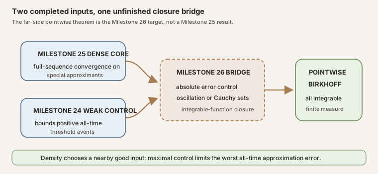
The intended implication is
[ \begin{aligned} &\text{dense pointwise-good core}
- \text{ absolute weak maximal control}\ &\hspace{2.2cm} \Longrightarrow \text{all integrable observables are pointwise-good}. \end{aligned} ]
That successor theorem uses finite total measure for this weak-bound route. It does not infer full pointwise convergence directly from the \(L^2\) mean theorem. It also does not call the invariant projection a conditional expectation; that identification belongs to another checked layer.
Continue with Pointwise Birkhoff from Maximal Control and Dense Good Functions to see the closure argument carried out. Chronology matters here: this chapter explains exactly what the RMT-25 module proves, even though the repository has since advanced beyond its stopping point.
Nonclaims
RMT-25 proves none of the following:
- the full-sequence almost-everywhere pointwise Birkhoff theorem for every \(L^2\) or \(L^1\) observable;
- that the pointwise limit of every dense-core representative equals the invariant projection representative;
- identification of \(P_Kf\) with conditional expectation;
- identification of fixed vectors with constants;
- preservation of the integral as a conclusion of the pointwise theorem;
- a unitary Koopman equivalence for noninvertible dynamics;
- a strong \(L^1\) maximal inequality;
- Kingman’s subadditive ergodic theorem;
- a Lyapunov exponent; or
- an Oseledets splitting.
References
B. O. Koopman, “Hamiltonian Systems and Transformation in Hilbert Space,” Proceedings of the National Academy of Sciences 17(5), 315–318 (1931), DOI 10.1073/pnas.17.5.315. Pages 315–316 construct the continuous-time composition operators used for the historical comparison.
J. von Neumann, “Proof of the Quasi-Ergodic Hypothesis,” Proceedings of the National Academy of Sciences 18(1), 70–82 (1932), DOI 10.1073/pnas.18.1.70, primary scan. Page 71 defines strong convergence as Hilbert-norm convergence; pages 72–74 give the interval-average projection theorem; pages 77–78 distinguish the subsequential almost-everywhere consequence.
G. D. Birkhoff, “Proof of the Ergodic Theorem,” Proceedings of the National Academy of Sciences 17(12), 656–660 (1931), DOI 10.1073/pnas.17.2.656, primary scan. Page 656 contrasts mean convergence with the pointwise problem; pages 659–660 state the continuous-time occupation result used for the historical boundary.
M. Keane and K. Petersen, “Easy and Nearly Simultaneous Proofs of the Ergodic Theorem and Maximal Ergodic Theorem,” IMS Lecture Notes-Monograph Series 48, 248–251 (2006), DOI 10.1214/074921706000000266, arXiv:math/0608251. Pages 248–250 provide the probability-space maximal-to-pointwise comparison used to plan the later maximal-closure module.
Mathlib 4.32.0, commit
81a5d257c8e410db227a6665ed08f64fea08e997,
MeanErgodic.lean, lines 47–108.
Lines 89–108 contain the continuous-linear-map orthogonal-projection theorem
specialized by RMT-25.
Mathlib 4.32.0,
LpSpace/Basic.lean, lines 559–633,
and
SimpleFuncDenseLp.lean, lines 519–526 and 648–675.
These are the pinned composition, representative, iterate, and simple-density
interfaces.
Mathlib 4.32.0,
Projection/Basic.lean, lines 121–169,
and
Projection/Submodule.lean, lines 81–92.
These supply projection membership, residual orthogonality, and the
double-orthogonal closure theorem.
Mathlib 4.32.0,
ConvergenceInMeasure.lean, lines 275–285 and 463–479.
These declarations formalize the norm-to-measure and
measure-to-almost-everywhere-subsequence ladder.
Nonlinear Dynamics in Lean,
KoopmanL2Mean.lean,
the checked RMT-25 implementation discussed throughout this chapter.