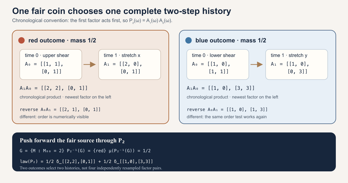
Start with two complete histories
Our sample space is the two-element set
\[ \Omega=\{\mathrm{red},\mathrm{blue}\}. \]Give each outcome probability \(1/2\). This assignment is a probability measure \(\mu\): the weights are nonnegative and add to one. We can imagine one fair coin toss, but the toss selects an entire two-step history at once. It does not toss a new coin independently at each time.
At time zero and time one, define these two-by-two integer matrices:
\[ \begin{array}{c|cc} \omega&A_0(\omega)&A_1(\omega)\\ \hline \mathrm{red}& \begin{bmatrix}1&1\\0&1\end{bmatrix}& \begin{bmatrix}2&0\\0&1\end{bmatrix}\\[9pt] \mathrm{blue}& \begin{bmatrix}1&0\\1&1\end{bmatrix}& \begin{bmatrix}1&0\\0&3\end{bmatrix}. \end{array} \]The map \(A_0\) sends an outcome to its time-zero matrix, and \(A_1\) does the same at time one. A map from a sample space into matrix space is a random matrix in the elementary sense used by this project. The adjective random describes dependence on \(\omega\); it does not mean that matrix multiplication itself is random.
For column-vector action, the time-zero matrix acts first. The chronological two-step product is therefore
\[ P_2(\omega)=A_1(\omega)A_0(\omega). \]Multiply the red history
\[ \begin{aligned} P_2(\mathrm{red}) &= \begin{bmatrix}2&0\\0&1\end{bmatrix} \begin{bmatrix}1&1\\0&1\end{bmatrix}\\[4pt] &= \begin{bmatrix} 2\cdot1+0\cdot0&2\cdot1+0\cdot1\\ 0\cdot1+1\cdot0&0\cdot1+1\cdot1 \end{bmatrix}\\[4pt] &= \begin{bmatrix}2&2\\0&1\end{bmatrix} =:R. \end{aligned} \]Reverse the order and the upper-right entry changes:
\[ A_0(\mathrm{red})A_1(\mathrm{red}) {} = \begin{bmatrix}2&1\\0&1\end{bmatrix} \ne R. \]This is why a one-by-one example is too weak for an order audit: scalar multiplication commutes, while these matrices do not.
Multiply the blue history
\[ \begin{aligned} P_2(\mathrm{blue}) &= \begin{bmatrix}1&0\\0&3\end{bmatrix} \begin{bmatrix}1&0\\1&1\end{bmatrix}\\[4pt] &= \begin{bmatrix}1&0\\3&3\end{bmatrix} =:B. \end{aligned} \]Again, the reverse order differs:
\[ A_0(\mathrm{blue})A_1(\mathrm{blue}) {} = \begin{bmatrix}1&0\\1&3\end{bmatrix} \ne B. \]The two values \(R\) and \(B\) are the complete image of \(P_2\).
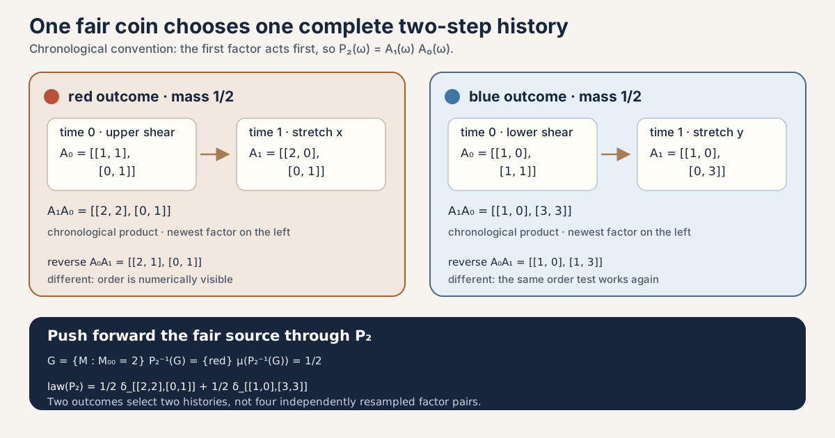
Compute a pushforward law atom by atom
An event is a measurable subset of the relevant space. On \(\Omega\), choose the full discrete measurable space, so all four subsets
\[ \varnothing,\quad \{\mathrm{red}\},\quad \{\mathrm{blue}\},\quad \Omega \]are events. Every function out of this finite discrete space is a measurable function . In particular, \(A_0\), \(A_1\), and \(P_2\) are measurable.
In the matrix target, consider
\[ G=\{M:M_{00}=2\}. \]To find the probability assigned to \(G\) by the product law, pull \(G\) back through the product map:
\[ \begin{aligned} P_2^{-1}(G) &=\{\omega:P_2(\omega)_{00}=2\}\\ &=\{\mathrm{red}\}. \end{aligned} \]Therefore
\[ \mu(P_2^{-1}(G))=\mu(\{\mathrm{red}\})=\frac12. \]The pushforward \((P_2)_*\mu\), also called the probability distribution or law of \(P_2\), is
\[ \mathcal L_\mu(P_2) {} = \frac12\delta_R+\frac12\delta_B. \]The symbol \(\delta_R\) is the Dirac point mass at \(R\): it assigns mass one to any measurable set containing \(R\) and mass zero otherwise. Thus the displayed formula is an atom-by-atom ledger:
| Target matrix | Preimage under \(P_2\) | Source mass | Product-law mass |
|---|---|---|---|
| \(R=[[2,2],[0,1]]\) | \(\{\mathrm{red}\}\) | \(1/2\) | \(1/2\) |
| \(B=[[1,0],[3,3]]\) | \(\{\mathrm{blue}\}\) | \(1/2\) | \(1/2\) |
| Any other matrix | \(\varnothing\) | \(0\) | \(0\) |
If two outcomes produced the same matrix, their source masses would merge at one target atom. At horizon zero, both outcomes produce the identity, so the law is
\[ \frac12\delta_I+\frac12\delta_I=\delta_I, \]not two distinguishable identity atoms. Pushforward laws remember output values and total mass at those values; they do not remember which outcomes collided there.
Under this fair measure, the only null set is the empty set. Consequently, “almost everywhere” and “everywhere” happen to agree for this toy space. The checked project theorem uses ordinary measurability anyway, so it works uniformly for every source measure rather than relying on this finite accident.
Three near-misses, three different questions
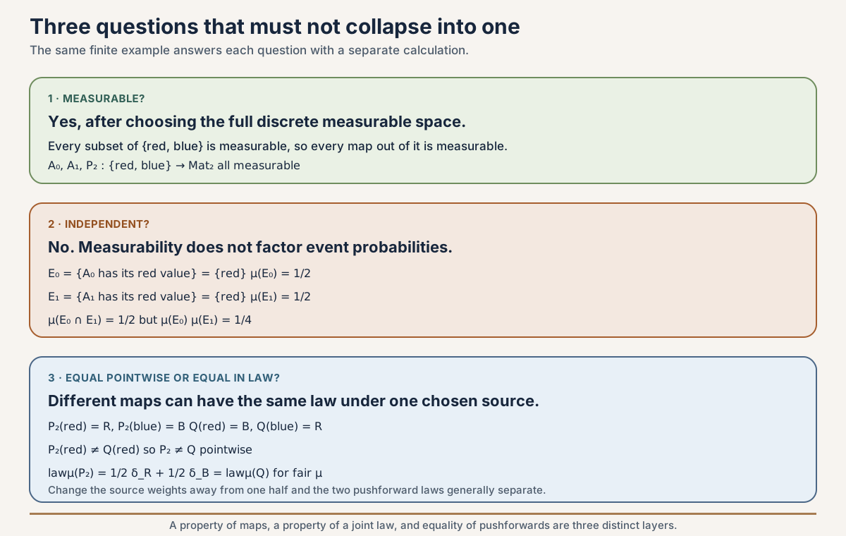
Measurability, independence, and equality in law are not interchangeable. The same two-outcome model separates them exactly.
Measurability does not imply independence
Define the factor events
\[ \begin{aligned} E_0&=\{\omega:A_0(\omega)=A_0(\mathrm{red})\} =\{\mathrm{red}\},\\ E_1&=\{\omega:A_1(\omega)=A_1(\mathrm{red})\} =\{\mathrm{red}\}. \end{aligned} \]Both factor maps are measurable. Yet
\[ \mu(E_0\cap E_1)=\frac12 \quad\text{while}\quad \mu(E_0)\mu(E_1)=\frac12\cdot\frac12=\frac14. \]The required factorization fails, so \(A_0\) and \(A_1\) are not independent . A shared outcome variable does not by itself imply dependence; the displayed unequal event probabilities establish dependence for this finite model.
Equality in law does not imply pointwise equality
Define another matrix-valued map \(Q\) by swapping the two outputs:
\[ Q(\mathrm{red})=B, \qquad Q(\mathrm{blue})=R. \]Then \(Q(\mathrm{red})\ne P_2(\mathrm{red})\), so \(Q\ne P_2\) as functions. But the fair source gives both atoms weight \(1/2\), hence
\[ \mathcal L_\mu(Q) =\frac12\delta_B+\frac12\delta_R =\mathcal L_\mu(P_2). \]This equality depends on the chosen source. If red had probability \(3/4\) and blue probability \(1/4\), \(P_2\) would place mass \(3/4\) on \(R\), whereas \(Q\) would place mass \(1/4\) there.
Type the finite ledger in Lean with Std
The general project theorem is a full project check: it imports Mathlib and
may require substantial disk space and memory. The exact two-outcome
arithmetic is a standalone tutorial for a normal macOS or Linux computer.
Save the following byte-for-byte as
/tmp/MeasurableFiniteProducts2.lean:
import Std

namespace MeasurableFiniteProducts2

structure Mat2 where
  a00 : Int
  a01 : Int
  a10 : Int
  a11 : Int
deriving Repr, DecidableEq, BEq

def identity : Mat2 :=
  ⟨1, 0, 0, 1⟩

def mul (A B : Mat2) : Mat2 :=
  ⟨A.a00 * B.a00 + A.a01 * B.a10,
   A.a00 * B.a01 + A.a01 * B.a11,
   A.a10 * B.a00 + A.a11 * B.a10,
   A.a10 * B.a01 + A.a11 * B.a11⟩

/-- The input list is chronological: the first matrix acts first. -/
def forwardProduct (factors : List Mat2) : Mat2 :=
  factors.foldl (fun earlier newest => mul newest earlier) identity

inductive Outcome where
  | red
  | blue
deriving Repr, DecidableEq, BEq

def outcomes : List Outcome :=
  [.red, .blue]

def A0 : Outcome → Mat2
  | .red  => ⟨1, 1, 0, 1⟩
  | .blue => ⟨1, 0, 1, 1⟩

def A1 : Outcome → Mat2
  | .red  => ⟨2, 0, 0, 1⟩
  | .blue => ⟨1, 0, 0, 3⟩

def product2 (ω : Outcome) : Mat2 :=
  forwardProduct [A0 ω, A1 ω]

def reversed2 (ω : Outcome) : Mat2 :=
  forwardProduct [A1 ω, A0 ω]

def preimage (f : Outcome → Mat2) (event : Mat2 → Bool) : List Outcome :=
  outcomes.filter (fun ω => event (f ω))

def topLeftIsTwo (M : Mat2) : Bool :=
  M.a00 == 2

def fairMass (event : Outcome → Bool) : Rat :=
  ((outcomes.filter event).length : Rat) / 2

def atomWeight (f : Outcome → Mat2) (target : Mat2) : Rat :=
  fairMass (fun ω => f ω == target)

def zeroProduct : Outcome → Mat2 :=
  fun _ => identity

def swappedProduct : Outcome → Mat2
  | .red  => product2 .blue
  | .blue => product2 .red

def firstFactorIsRed (ω : Outcome) : Bool :=
  A0 ω == A0 .red

def secondFactorIsRed (ω : Outcome) : Bool :=
  A1 ω == A1 .red

#eval product2 .red
#eval product2 .blue
#eval reversed2 .red
#eval reversed2 .blue
#eval preimage product2 topLeftIsTwo
#eval [(product2 .red, atomWeight product2 (product2 .red)),
       (product2 .blue, atomWeight product2 (product2 .blue))]
#eval atomWeight zeroProduct identity
#eval (fairMass firstFactorIsRed,
       fairMass secondFactorIsRed,
       fairMass (fun ω => firstFactorIsRed ω && secondFactorIsRed ω))
#eval [(atomWeight product2 (product2 .red),
        atomWeight swappedProduct (product2 .red)),
       (atomWeight product2 (product2 .blue),
        atomWeight swappedProduct (product2 .blue))]

example : forwardProduct [] = identity := by decide
example : forwardProduct [A0 .red] = A0 .red := by decide
example : product2 .red = ⟨2, 2, 0, 1⟩ := by decide
example : product2 .blue = ⟨1, 0, 3, 3⟩ := by decide
example : preimage product2 topLeftIsTwo = [.red] := by decide
example : atomWeight product2 (product2 .red) = (1 : Rat) / 2 := by native_decide
example : atomWeight product2 (product2 .blue) = (1 : Rat) / 2 := by native_decide
example : atomWeight zeroProduct identity = 1 := by native_decide
example : fairMass (fun ω => firstFactorIsRed ω && secondFactorIsRed ω) ≠
    fairMass firstFactorIsRed * fairMass secondFactorIsRed := by native_decide
example : swappedProduct .red ≠ product2 .red := by decide
example : atomWeight product2 (product2 .red) =
    atomWeight swappedProduct (product2 .red) := by native_decide
example : atomWeight product2 (product2 .blue) =
    atomWeight swappedProduct (product2 .blue) := by native_decide

end MeasurableFiniteProducts2
Load the pinned toolchain environment if needed, then type:
source "$HOME/.elan/env"
elan run leanprover/lean4:v4.32.0 lean \
  /tmp/MeasurableFiniteProducts2.lean
This exact worksheet was executed successfully with Lean 4.32.0. It printed:
{ a00 := 2, a01 := 2, a10 := 0, a11 := 1 }
{ a00 := 1, a01 := 0, a10 := 3, a11 := 3 }
{ a00 := 2, a01 := 1, a10 := 0, a11 := 1 }
{ a00 := 1, a01 := 0, a10 := 1, a11 := 3 }
[MeasurableFiniteProducts2.Outcome.red]
[({ a00 := 2, a01 := 2, a10 := 0, a11 := 1 }, (1 : Rat)/2), ({ a00 := 1, a01 := 0, a10 := 3, a11 := 3 }, (1 : Rat)/2)]
1
((1 : Rat)/2, (1 : Rat)/2, (1 : Rat)/2)
[((1 : Rat)/2, (1 : Rat)/2), ((1 : Rat)/2, (1 : Rat)/2)]
Read the output from top to bottom. The first two matrices are \(R\) and \(B\). The next two are the reverse-order products. The singleton list is the preimage of \(G\). The weighted matrix list is the two-atom pushforward ledger. The next output, \(1\), records that the red and blue zero-horizon identity outcomes merge into one atom of total weight one. The triple \((1/2,1/2,1/2)\) records the two factor-event masses and their intersection, so it visibly fails the independence target \(1/4\). The last pairs show equal atom weights for \(P_2\) and the swapped map.
The symbols are deliberately elementary:
structure Mat2gives names to four integer entries.mul A Bimplements the four row-by-column formulas for \(AB\).foldlreads factors chronologically; its callback multiplies each newest factor on the left of the accumulated earlier product.inductive Outcomecreates exactly two constructors.filtercomputes a finite preimage by retaining outcomes whose output satisfies the event test.Ratkeeps the masses \(1/2\) exact.decideandnative_decideclose finite, computational propositions with kernel-checked proofs.
This worksheet checks the numerical ledger. It does not formalize measurable
spaces, Measure.map, complex Mathlib matrices, or the general
finite-product theorems below.
Consider a time-indexed family of random square matrices
\[ A_0,A_1,A_2,\ldots, \qquad A_j:\Omega\to M_\iota(\mathbb C). \]At one outcome \(\omega\), the first \(k\) factors become ordinary matrices and form the chronological product
\[ \Pi_k(\omega) {} = A_{k-1}(\omega)\cdots A_1(\omega)A_0(\omega). \]This expression is a matrix-valued function on the sample space. It is not yet a measure, and the notation does not prove that it is measurable. To reach a law, we need a precise chain:
- define the sample product pointwise;
- prove that only the factors in its finite prefix need to be measurable;
- transport a chosen source measure through the certified map;
- prove that this raw law has mass one when the source does; and
- optionally bundle the raw law and its mass-one evidence into a probability measure type.
The module
NonlinearDynamics.Random.MatrixProducts.MeasurableFiniteProducts
checks that complete chain at every finite horizon. It exposes one definition
and four theorems in a semiring-valued sample-algebra layer, then two
definitions and five theorems in a complex measurable-law layer. There are
twelve public declarations in total.
The result is deliberately finite. It adds no independence, stationarity, base transformation, cocycle structure, norm estimate, logarithm, or long-time limit. That narrowness is the point. Later random dynamics should build on a sample map and law whose finite meaning is already exact.
Choose a route up
| Route | Begin with | Destination |
|---|---|---|
| First encounter | Four layers in one picture | Separate factors, samples, laws, and bundled probability laws |
| Algebra route | Evaluate first, multiply second | Derive zero, successor, one-step, and split identities |
| Measure route | Measurability uses exactly one prefix | Understand the finite induction and its hypotheses |
| Lean route | The complete declaration map | Audit all twelve names and assumptions |
| Boundary route | Empty dimension is not an exception | See why no positive-dimension hypothesis appears |
| Law route | A law is a certified pushforward | Keep Mathlib’s fallback from becoming an assumption |
| Probability route | Raw mass-one theorem versus bundled law | Distinguish a measure, evidence about it, and a subtype |
| Summit route | What has and has not been proved | Preserve every explicit nonclaim |
Learning objectives
By the summit, you should be able to:
- distinguish a time-indexed factor family from one pointwise product;
- expand the product at horizons zero, one, two, and three;
- explain why the newest factor is written on the left;
- derive the shifted finite-block split sample by sample;
- identify the five declarations that require only a semiring;
- state the exact prefix measurability hypothesis \(\forall j\lt k\);
- prove finite-product measurability by induction;
- explain why the measurable layer is scoped to complex matrices;
- explain why neither layer needs a nonempty coordinate type;
- distinguish ordinary measurability from Mathlib’s
almost-everywhere-measurable fallback for
Measure.map; - explain what evidence the
RandomMatrix.lawinterface requires; - compute the zero-step and one-step laws;
- state why the zero-step Dirac theorem needs a probability source;
- distinguish a raw measure with a mass-one theorem from a bundled
ProbabilityMeasure; - explain why coercing the wrapper changes no probabilities;
- map every claim to one of the twelve public declarations; and
- list the independence, cocycle, growth, and asymptotic conclusions that remain absent.
Four layers in one picture
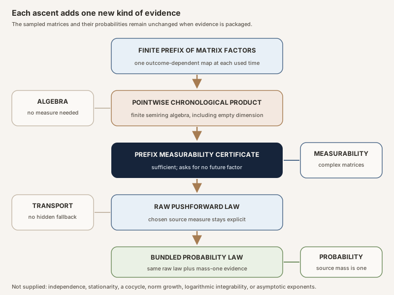
The four boxes are different mathematical types:
| Layer | Mathematical object | Lean-facing shape | What it records |
|---|---|---|---|
| Factor family | A map at each natural time | ℕ → RandomMatrix Ω ι ι ℂ | How one outcome selects every finite-time factor |
| Sample product | One matrix-valued map | RandomMatrix Ω ι ι ℂ | The ordered product at a chosen horizon |
| Raw law | A measure on matrix space | Measure (Matrix ι ι ℂ) | How source mass is distributed over product values |
| Bundled law | A raw law plus mass-one evidence | ProbabilityMeasure (Matrix ι ι ℂ) | The same law with probability status in its type |
A measurability proof is evidence connecting the first two rows to the third.
An IsProbabilityMeasure proof is evidence connecting the third row
to the fourth. Neither proof changes a sampled matrix or a probability value.
Base camp: fix the chronological convention
Let \(P_B(k)\) be the deterministic forward product of a matrix sequence \(B:\mathbb N\to M_\iota(\mathbb K)\):
\[ P_B(0)=I, \qquad P_B(k+1)=B_kP_B(k). \]The first cases are
\[ \begin{aligned} P_B(0)&=I,\\ P_B(1)&=B_0,\\ P_B(2)&=B_1B_0,\\ P_B(3)&=B_2B_1B_0. \end{aligned} \]The horizon counts factors. Horizon \(k\) reads indices \(0,\ldots,k-1\). For column vectors, \(B_0\) acts first and therefore appears furthest to the right. The forward matrix product entry and Ordered Finite Matrix Products and Operator-Norm Growth develop this deterministic layer in full.
The present module does not invent a second order convention. It evaluates the existing deterministic definition at each outcome.
Camp one: evaluate first, multiply second
For a time-indexed family \(A_j:\Omega\to M_\iota(\mathbb K)\), define
\[ \Pi_k(\omega) {} = P_{j\mapsto A_j(\omega)}(k). \]Lean calls this map sampleForwardProduct A k:
def sampleForwardProduct
    (A : ℕ → RandomMatrix Ω ι ι 𝕜) (k : ℕ) :
    RandomMatrix Ω ι ι 𝕜 :=
  fun ω => forwardProduct (fun j => A j ω) k
This is a pointwise lift. First fix \(\omega\). Then \(j\mapsto A_j(\omega)\) is an ordinary matrix sequence, so the deterministic product can consume it. The result varies with \(\omega\), producing another matrix-valued map.
The entire section assumes:
- \(\iota\) is a finite index type;
- equality on \(\iota\) is decidable; and
- \(\mathbb K\) is a semiring.
Finiteness and decidable equality support the finite sums in matrix multiplication. A semiring supplies the algebra used by matrices. There is no sample-space measurable structure, source measure, topology, norm, order, subtraction, division, or probability assumption in this layer.
That assumption ledger matters. The name RandomMatrix is an
abbreviation for a function into matrix space. It does not force probability
structure into every theorem that uses the name.
Camp two: inherit the finite algebra pointwise
Because the definition delegates to forwardProduct, four
identities follow outcome by outcome.
Zero horizon
\[ \Pi_0(\omega)=I. \]The empty product is the constant identity map. Lean publishes
sampleForwardProduct_zero, and the proof is reflexivity.
Successor horizon
\[ \Pi_{k+1}(\omega)=A_k(\omega)\Pi_k(\omega). \]sampleForwardProduct_succ A ksampleForwardProductis the matrix-valued function \(\omega\mapsto\Pi_k(\omega)\).- The suffix
_succannounces the successor horizonk + 1. - The first explicit argument
Ais the whole time-indexed factor family;kselects the newest index. - In the theorem’s result,
fun ω =>means “at every outcome \(\omega\),” and*is matrix multiplication. - The newest factor is on the left because \(A_0\) acts first on a column vector.
The result is definitional: after unfolding the recursion, the proof closes with
rfl.
One step
\[ \Pi_1=A_0. \]This is equality of functions, not merely equality at one outcome.
sampleForwardProduct_one proves it by function extensionality and
simplification of the deterministic product.
Split after a finite prefix
Let the early block contain \(m\) factors and the later block contain \(k\) factors. Define the shifted family \(A^{(m)}_j=A_{m+j}\). Then
\[ \Pi_{m+k}(\omega) {} = \Pi^{(m)}_k(\omega)\Pi_m(\omega). \]The earlier block is on the right because it acts first. The shifted later
block is on the left because it acts second. The theorem
sampleForwardProduct_add uses function extensionality and then
applies forwardProduct_add at the chosen outcome.
sampleForwardProduct_add A m kaddrefers to the horizon decompositionm + k.fun j => A (m + j)is the shifted family \(A^{(m)}\); its local time zero is global time \(m\).sampleForwardProduct … k ωevaluates the later block at the same outcome as the earlier block.- The rightmost
sampleForwardProduct A m ωacts first. - The equality is pointwise algebra. It does not factor the distribution of the two blocks.
Full project check. Put these lines in a temporary project scratch file after installing the repository’s pinned dependencies:
import NonlinearDynamics.Random.MatrixProducts.MeasurableFiniteProducts

#check NonlinearDynamics.Random.MatrixProducts.sampleForwardProduct_succ
#check NonlinearDynamics.Random.MatrixProducts.sampleForwardProduct_add
The first check exposes newest-factor-left recursion. The second exposes the shifted later family and block order. The command below checks the exact committed module with its pinned project dependencies.
cd formalization
lake env lean -DwarningAsError=true NonlinearDynamics/Random/MatrixProducts/MeasurableFiniteProducts.lean
Resource note: this exact file uses the repository's
pinned Lean and Mathlib dependencies. Initial project setup can require
substantial disk space and build time. For a lightweight first step on
macOS or Linux, use the page's standalone Lean-core or Std
tutorial.
No measurability is needed for any of these equations. They are finite algebra of functions.
Read the split through the two-outcome expedition
Return to the opening matrices and split the horizon-two product after one step. Here \(m=1\) and \(k=1\). The shifted later family begins at \(A_1\), so
\[ \Pi_2(\omega) {} = \underbrace{\Pi^{(1)}_1(\omega)}_{A_1(\omega)} \underbrace{\Pi_1(\omega)}_{A_0(\omega)} =A_1(\omega)A_0(\omega). \]At red this recovers \(R=[[2,2],[0,1]]\); at blue it recovers \(B=[[1,0],[3,3]]\). Omitting the shift would reuse \(A_0\) in the later block. Reversing the block order would produce the two reverse matrices already computed. The concrete ledger therefore detects both common implementation mistakes.
Camp three: measurability uses exactly one prefix
Equip \(\Omega\) with a measurable space. For a fixed horizon \(k\), the checked hypothesis is
\[ h_A:\forall j\lt k,\quad A_j\text{ is measurable}. \]The quantifier ends at \(k\). The sample product \(\Pi_k\) never reads a factor at time \(k\) or later, so future measurability is irrelevant.
This hypothesis is scope-exact: it asks only about indices the definition reads. It is a sufficient condition, not an if-and-only-if characterization. For example, a nonmeasurable earlier factor could be annihilated by a later constant zero matrix, leaving a measurable zero product. The checked theorem does not claim that measurability of \(\Pi_k\) forces every used factor to be measurable.
The theorem is:
theorem measurable_sampleForwardProduct
    (A : ℕ → RandomMatrix Ω ι ι ℂ)
    (k : ℕ) (hA : ∀ j < k, Measurable (A j)) :
    Measurable (sampleForwardProduct A k)
measurable_sampleForwardProduct A k hAhAis the proof of the bounded statement∀ j < k, Measurable (A j).∀means “for every,” whilej < krestricts that quantifier to the finite prefix.Measurable (A j)is ordinary map measurability, not almost-everywhere measurability relative to one measure.- The conclusion names
sampleForwardProduct A k, the whole matrix-valued sample map. - The scalar type is exactly \(\mathbb C\) in this theorem. The earlier algebra declarations are more general, but this checked measurable interface is not.
The proof is induction on \(k\).
Base case
At horizon zero, sampleForwardProduct_zero rewrites the map as
the constant identity. RandomMatrix.measurable_const proves that
this constant matrix-valued function is measurable. The prefix premise is
vacuous because no natural number is less than zero.
Successor case
At horizon \(k+1\),
\[ \Pi_{k+1}(\omega)=A_k(\omega)\Pi_k(\omega). \]The premise supplies measurability of \(A_k\) from
\(k\lt k+1\). It also restricts to every earlier \(j\lt k\), allowing the
induction hypothesis to prove that \(\Pi_k\) is measurable.
RandomMatrix.measurable_mul then proves measurability of the
pointwise matrix product.
The proof architecture mirrors the mathematics exactly:
| Recursive product branch | Measurability ingredient |
|---|---|
| Empty identity product | Constant maps are measurable |
| New factor times previous product | Each factor is measurable, induction handles the prefix, multiplication is measurable |
The project theorem and the matrix-multiplication interface it consumes can be inspected together:
import NonlinearDynamics.Random.MatrixProducts.MeasurableFiniteProducts

#check NonlinearDynamics.Random.MatrixProducts.measurable_sampleForwardProduct
#check NonlinearDynamics.Random.RandomMatrix.measurable_mul
The first type displays the bounded prefix premise. The second confirms the induction step’s pointwise multiplication rule. Run the authoritative module with the full project command below.
cd formalization
lake env lean -DwarningAsError=true NonlinearDynamics/Random/MatrixProducts/MeasurableFiniteProducts.lean
Resource note: this exact file uses the repository's
pinned Lean and Mathlib dependencies. Initial project setup can require
substantial disk space and build time. For a lightweight first step on
macOS or Linux, use the page's standalone Lean-core or Std
tutorial.
Why complex matrices?
The semiring sample layer is fully general because it uses only finite matrix algebra. The measurable theorem is stated for \(\mathbb C\), where the project already has a checked measurable-space interface for finite complex matrices and measurable multiplication.
This scope is not a theorem that complex scalars are mathematically necessary. It is the exact interface proved in this module. A future generalization would need suitable measurable structures and measurable multiplication for the chosen scalar type.
Camp four: empty dimension is not an exception
No Nonempty ι assumption appears. If \(\iota\) is empty, a matrix
\(\iota\to\iota\to\mathbb C\) has no entries and therefore exactly one value.
That unique matrix is the identity, and multiplying it by itself returns it.
The sample algebra still works:
\[ \Pi_k(\omega)=I \]for every \(k\) and every \(\omega\). The map is constant and measurable. Under a probability source, its law is the point mass at the unique matrix.
This boundary contrasts with the deterministic maximum-row-sum norm layer. There, positive dimension is used to normalize the identity matrix to norm one. The present module performs no norm calculation. Finite matrix algebra, measurability, and pushforward transport remain valid in empty dimension.
Empty dimension is therefore supported by design, not repaired by a special fallback.
Camp five: a law is a certified pushforward
Let \(\mu\) be any measure on \(\Omega\). Given the exact prefix proof \(h_A\), the module defines
\[ \operatorname{Law}_{\mu,A,k,h_A} {} = (\Pi_k)_*\mu. \]In Lean:
noncomputable def forwardProductLaw
    (μ : Measure Ω)
    (A : ℕ → RandomMatrix Ω ι ι ℂ)
    (k : ℕ) (hA : ∀ j < k, Measurable (A j)) :
    Measure (Matrix ι ι ℂ) :=
  RandomMatrix.law (sampleForwardProduct A k)
    (measurable_sampleForwardProduct A k hA) μ
forwardProductLaw μ A k hAμis the sourceMeasure Ω; changing it can change the output law even whenAis unchanged.Aandkdetermine the sample mapsampleForwardProduct A k.hAproves exactly the finite-prefix premise used to derive product measurability.- Inside the definition,
RandomMatrix.lawis the project’s explicit-evidence interface toMeasure.map. - The resulting type is the raw
Measure (Matrix ι ι ℂ). It does not storehAas a data field.
The source measure is explicit. The factor family alone cannot determine a law because different measures on the same outcome space can assign different weights to the same product values.
The measurability proof is also explicit. It certifies the map before the law interface transports \(\mu\). This is the sense in which the pushforward law is proof-carrying: the definition call receives evidence establishing the map’s mathematical precondition.
The result itself is still a raw Measure. It is not a dependent
record that exposes the measurability proof as a field. Proof irrelevance also
means that choosing a different proof of the same proposition cannot change
the transported measure.
Why the certificate matters in Mathlib
Mathematically, the pushforward identity
\[ (f_*\mu)(B)=\mu(f^{-1}(B)) \]is used for measurable target sets when \(f\) is suitably measurable.
Mathlib defines Measure.map f μ as a total function. When \(f\)
is not almost everywhere measurable with respect to \(\mu\), the definition
falls back to the zero measure. This design keeps terms total, but it creates
a semantic trap: an unproved map expression still elaborates, while its value
may no longer represent the intended transported probability.
RandomMatrix.law requires an ordinary measurability proof. The
finite-product definition supplies that proof from \(h_A\), so later law
identities do not silently rely on the zero fallback. Ordinary measurability
is stronger than almost-everywhere measurability and is stable across every
source measure.
The product-law constructor and its predecessor law interface can be inspected side by side:
import NonlinearDynamics.Random.MatrixProducts.MeasurableFiniteProducts

#check NonlinearDynamics.Random.MatrixProducts.forwardProductLaw
#check NonlinearDynamics.Random.RandomMatrix.law
#check NonlinearDynamics.Random.RandomMatrix.law_apply
The first two declaration types display where ordinary measurability evidence enters. The third is the checked preimage-evaluation theorem matching the opening ledger. The full project command below checks the authoritative module.
cd formalization
lake env lean -DwarningAsError=true NonlinearDynamics/Random/MatrixProducts/MeasurableFiniteProducts.lean
Resource note: this exact file uses the repository's
pinned Lean and Mathlib dependencies. Initial project setup can require
substantial disk space and build time. For a lightweight first step on
macOS or Linux, use the page's standalone Lean-core or Std
tutorial.
Camp six: calibrate the law at zero and one step
The first two horizons catch most convention errors.
Zero-step law
If \(\mu\) is a probability measure, then
\[ \operatorname{Law}_{\mu,A,0}=\delta_I. \]The sample map at horizon zero is constant at the identity. Pushing a
probability measure through a constant map puts all unit mass at that value.
Lean names the theorem forwardProductLaw_zero.
forwardProductLaw_zero μ A hA- The hidden typeclass argument
[IsProbabilityMeasure μ]supplies \(\mu(\Omega)=1\). - The numeral
0selects the empty product. hA : ∀ j < 0, Measurable (A j)has no cases; it is present only because the law interface uses one uniform evidence shape.Measure.dirac 1is the right side of the theorem. Here1is the matrix identity, inferred from the target type.- If several sample outcomes all map to that identity, their masses merge into this single atom, as in the opening two-outcome calculation.
The typeclass hypothesis [IsProbabilityMeasure μ] is essential
for this exact unit Dirac formula. For a general measure, a constant
pushforward retains the source’s total mass. A source of mass \(c\) would
produce \(c\delta_I\), not necessarily \(\delta_I\).
The theorem still receives
hA : ∀ j < 0, Measurable (A j)
because the law definition has a uniform evidence argument. This premise is vacuous.
One-step law
At horizon one, the sample product is \(A_0\), so
\[ \operatorname{Law}_{\mu,A,1} {} = \mathcal L_\mu(A_0). \]Lean’s forwardProductLaw_one states the right side with
RandomMatrix.law and the extracted proof
hA 0 Nat.zero_lt_one.
No probability hypothesis is needed. The identity compares two pushforwards of the same raw measure by the same map. Whatever total mass \(\mu\) has, both sides retain it.
The zero and one formulas test different things:
| Calibration | What it checks |
|---|---|
| Zero law is Dirac at identity | Empty-product convention and probability mass normalization |
| One law equals the first factor law | Horizon indexing and factor order |
These exact calibration declarations distinguish the assumptions at horizons zero and one:
import NonlinearDynamics.Random.MatrixProducts.MeasurableFiniteProducts

#check NonlinearDynamics.Random.MatrixProducts.forwardProductLaw_zero
#check NonlinearDynamics.Random.MatrixProducts.forwardProductLaw_one
The zero theorem carries a source probability typeclass; the one-step equality does not. Use the full project command below to check their authoritative types and proofs.
cd formalization
lake env lean -DwarningAsError=true NonlinearDynamics/Random/MatrixProducts/MeasurableFiniteProducts.lean
Resource note: this exact file uses the repository's
pinned Lean and Mathlib dependencies. Initial project setup can require
substantial disk space and build time. For a lightweight first step on
macOS or Linux, use the page's standalone Lean-core or Std
tutorial.
Camp seven: raw mass-one theorem versus bundled law
The definition forwardProductLaw accepts an arbitrary raw
Measure Ω. When the source has total mass one, measurable
pushforward preserves that mass. The theorem
theorem forwardProductLaw_isProbabilityMeasure
    (μ : Measure Ω) [IsProbabilityMeasure μ]
    (A : ℕ → RandomMatrix Ω ι ι ℂ) (k : ℕ)
    (hA : ∀ j < k, Measurable (A j)) :
    IsProbabilityMeasure (forwardProductLaw μ A k hA)
forwardProductLaw_isProbabilityMeasure μ A k hAIsProbabilityMeasureis a proposition about the raw output measure; it is not a second measure.- Lean finds the source hypothesis through
[IsProbabilityMeasure μ]. μ A k hAare the same source, factor family, horizon, and prefix certificate used byforwardProductLaw.- The theorem delegates to
RandomMatrix.law_isProbabilityMeasureafter supplying the derived product measurability proof. - No division or normalization occurs. Pushforward preserves the source’s already-unit total mass.
This records the result as a proposition and typeclass-bearing proof. It does not construct a different measure.
The next definition starts from a bundled source
μ : ProbabilityMeasure Ω and packages the target:
noncomputable def forwardProductProbabilityLaw
    (μ : ProbabilityMeasure Ω)
    (A : ℕ → RandomMatrix Ω ι ι ℂ) (k : ℕ)
    (hA : ∀ j < k, Measurable (A j)) :
    ProbabilityMeasure (Matrix ι ι ℂ)
A ProbabilityMeasure α contains:
- a raw
Measure α; and - evidence that its total mass is one.
The constructor uses forwardProductLaw as the raw component and
forwardProductLaw_isProbabilityMeasure as its evidence.
Finally,
coe_forwardProductProbabilityLaw proves that forgetting the
wrapper recovers the raw law:
The proof is reflexivity. The wrapper is transparent by construction. It adds a guarantee to the type and no renormalization, conditioning, or change of sample weights.
coe_forwardProductProbabilityLaw μ A k hAforwardProductProbabilityLawstarts withμ : ProbabilityMeasure Ω, so source mass one is already in the input type.- The double coercion visible in the full theorem converts the bundled target
back to
Measure (Matrix ι ι ℂ). coe_in the theorem name signals this forgetful comparison.- The right side calls
forwardProductLawon the raw measure underlying \(\mu\). - The proof is
rfl, confirming that packaging added evidence but changed no atom and no weight.
The mass-one theorem, bundled constructor, and forgetful equality form the final interface:
import NonlinearDynamics.Random.MatrixProducts.MeasurableFiniteProducts

#check NonlinearDynamics.Random.MatrixProducts.forwardProductLaw_isProbabilityMeasure
#check NonlinearDynamics.Random.MatrixProducts.forwardProductProbabilityLaw
#check NonlinearDynamics.Random.MatrixProducts.coe_forwardProductProbabilityLaw
The first result is evidence about a raw measure, the second is a bundled probability measure, and the third proves their underlying measures coincide. The exact project file is checked by the full project command below.
cd formalization
lake env lean -DwarningAsError=true NonlinearDynamics/Random/MatrixProducts/MeasurableFiniteProducts.lean
Resource note: this exact file uses the repository's
pinned Lean and Mathlib dependencies. Initial project setup can require
substantial disk space and build time. For a lightweight first step on
macOS or Linux, use the page's standalone Lean-core or Std
tutorial.
The complete declaration map
The module exposes exactly twelve public declarations.
| Declaration | Layer | Exact role |
|---|---|---|
sampleForwardProduct | Semiring sample algebra | Evaluates the factor family at one outcome and forms the deterministic forward product |
sampleForwardProduct_zero | Semiring sample algebra | The zero-horizon sample map is constant at identity |
sampleForwardProduct_succ | Semiring sample algebra | The newest sampled factor is multiplied on the left |
sampleForwardProduct_one | Semiring sample algebra | The one-step sample product is the time-zero factor map |
sampleForwardProduct_add | Semiring sample algebra | A long sample product splits into a shifted later block times the earlier block |
measurable_sampleForwardProduct | Complex measurable map | Exact-prefix factor measurability implies sample-product measurability |
forwardProductLaw | Raw measure | Uses the certified sample product in RandomMatrix.law |
forwardProductLaw_zero | Raw measure calibration | Under a probability source, the empty product law is Dirac at identity |
forwardProductLaw_one | Raw measure calibration | The one-step product law is the law of the time-zero factor |
forwardProductLaw_isProbabilityMeasure | Mass-one evidence | A probability source gives the raw product law total mass one |
forwardProductProbabilityLaw | Bundled measure | Packages the raw law and mass-one evidence as a probability measure |
coe_forwardProductProbabilityLaw | Interface coherence | Coercion of the bundled law recovers the raw law definitionally |
The five declarations in the first layer work over any semiring and do not
require a measurable space on \(\Omega\). The remaining seven use a measurable
sample space and complex matrices. The zero-law and raw mass-one theorem add a
probability hypothesis on the raw source. The bundled-law constructor encodes
that source hypothesis in ProbabilityMeasure Ω.
No declaration assumes Nonempty ι.
Proof architecture
The proof scripts are short because earlier interfaces carry the mathematical weight:
| Goal | Main ingredients |
|---|---|
| Zero and successor sample equations | Definitional reduction |
| One-step sample equation | Function extensionality and deterministic simplification |
| Shifted split | Function extensionality and forwardProduct_add |
| Product measurability | Natural-number induction, measurable constant, measurable multiplication |
| Raw law | RandomMatrix.law applied to the proved measurable product |
| Zero law | Constant-map pushforward under a probability source |
| One law | One-step function identity and the same pushforward |
| Raw mass one | RandomMatrix.law_isProbabilityMeasure |
| Bundled law | Pair the raw measure with its mass-one proof |
| Coercion theorem | Reflexivity |
Short code is not shallow mathematics. The module is concise because the deterministic product convention, finite matrix measurable structure, measurable multiplication, pushforward law, and probability-measure subtype were each established earlier.
Why this finite layer matters for dynamics and physics
Finite products appear before every asymptotic theory.
Random linear recurrences
A random recurrence
\[ x_{j+1}(\omega)=A_j(\omega)x_j(\omega) \]has finite solution
\[ x_k(\omega)=\Pi_k(\omega)x_0 \]when the initial state is deterministic. Before asking for expected growth or almost-sure stability, \(\Pi_k\) must be a measurable random matrix. The present theorem supplies that map-level foundation for a finite prefix.
Tangent dynamics
For a differentiable nonlinear system, derivatives along an orbit multiply in chronological order. If the system or initial data is random, those derivative matrices become outcome-dependent. A measurable finite-product interface is a prerequisite for probabilistic questions about finite-time tangent propagators.
This module does not connect \(A_j\) to derivatives, prove a chain rule, or define a nonlinear orbit. It only provides the matrix-product layer such a bridge would consume.
Transfer and scattering chains
Products of transfer matrices describe finite chains in wave propagation, statistical mechanics, and disordered media. A finite chain has a sample-dependent transfer matrix and hence a law when the disorder variables are measurable. Independence or a particular disorder distribution is model data, not a consequence of multiplication.
The road to Lyapunov exponents
Long-time random matrix theory studies quantities such as
\[ \lim_{k\to\infty}\frac{1}{k}\log\lVert\Pi_k(\omega)\rVert. \]That expression requires far more than a measurable finite product:
- a norm and usually invertibility or controlled degeneracy;
- logarithmic integrability;
- a stationary or measure-preserving base dynamics;
- a cocycle identity over that base;
- an almost-sure limiting theorem; and
- for invariant splittings, the full hypotheses of a multiplicative ergodic theorem.
RMT-12 proves none of those bullets. It ensures that the finite random object and its law are available without guessing the earlier interface.
Common wrong turns
Calling the factor family a product law
The family \(A\) is a sequence of matrix-valued functions. The product \(\Pi_k\) is another function. Its law is a measure formed only after choosing \(\mu\) and proving measurability.
Reversing chronological order
For column action, \(A_0\) acts first and is written on the right. The successor product is \(A_k\Pi_k\), not \(\Pi_kA_k\).
Forgetting the shift in the split
The later block begins at \(A_m\), not \(A_0\). Omitting \(j\mapsto A_{m+j}\) duplicates the wrong time segment.
Requiring every future factor to be measurable
Horizon \(k\) reads only \(A_0,\ldots,A_{k-1}\). The checked premise is exact in scope: it asks only for that prefix. It is a sufficient hypothesis, not a claim that product measurability logically forces measurability of every used factor.
Treating Measure.map as an unconditional probability law
Mathlib’s operation is total and has a zero-measure fallback outside its almost-everywhere-measurable regime. The project supplies ordinary measurability explicitly before calling the law interface.
Assuming a law definition proves mass one
forwardProductLaw accepts an arbitrary raw source measure. Its
mass matches the source’s mass. Probability status is a separate theorem with
a source probability hypothesis.
Reading the bundled law as renormalization
forwardProductProbabilityLaw wraps an already mass-one raw law.
Its coercion theorem is reflexive. No weights change.
Adding an unsupported independence assumption
Measurability of each factor does not imply that factors are independent, identically distributed, or stationary. Their joint dependence can be arbitrary.
Adding positive dimension from the norm chapter
The norm chapter needs positive dimension for identity-norm normalization. This sample and law layer does not use a norm and supports an empty coordinate type.
Reading finite laws as asymptotics
A law for every chosen finite \(k\) is not a limit theorem. It does not produce a Lyapunov exponent, invariant splitting, central limit theorem, or universal spectral law.
Exercises from trailhead to summit
Trailhead
- Expand \(\Pi_k(\omega)\) for \(k=0,1,2,3,4\).
- For a column vector, add parentheses that expose the action order at horizon three.
- Explain why
sampleForwardProduct_zerois an equality of functions. - Verify the two-outcome example at every displayed horizon.
Mid-mountain
- Prove
sampleForwardProduct_oneon paper from the recursive definition. - Expand both sides of the split law for \(m=2\) and \(k=3\).
- Write the exact factor indices used by \(\Pi_k\), then justify the bound \(j\lt k\) in the measurability hypothesis.
- Reproduce the measurability induction. Identify where \(k\lt k+1\) and \(j\lt k\Rightarrow j\lt k+1\) enter.
- Construct two fully dependent measurable factors on a two-point space and compute their two-step law.
- Give two different source probability measures on the same outcome space and show that the same sample product map has two different laws.
Summit
- For a raw source measure of finite mass \(c\), compute the pushforward of the zero-step product and explain why the checked Dirac theorem assumes \(c=1\).
- Explain, without using the word wrapper, the type difference between
Measure αwith an externalIsProbabilityMeasureproof andProbabilityMeasure α. - Describe Mathlib’s nonmeasurable-map fallback and explain why the explicit proof argument rules it out for this construction.
- Prove that every finite product in empty matrix dimension is the unique identity matrix.
- Design a later measurable cocycle structure. List the base map, cocycle law, source measure, and invariance hypotheses absent here.
- State a plausible finite-time norm random variable built from \(\Pi_k\). List the additional norm measurability and integrability results needed before taking its expectation.
- State the hypotheses of a multiplicative ergodic theorem that cannot be inferred from these twelve declarations.
Reproduce the checked slice
There are two deliberately separate resource lanes.
On a normal Mac or Linux host, rerun only the bounded Std
worksheet from the opening:
elan run leanprover/lean4:v4.32.0 lean \
  /tmp/MeasurableFiniteProducts2.lean
That command checks exact integer matrix arithmetic, finite preimages, rational
atom weights, the dependence witness, and the same-law/different-map example.
It imports Std, not Mathlib.
For the full project check, install the repository’s pinned Lean and Mathlib dependencies. From the repository root, type:
cd formalization
lake env lean NonlinearDynamics/Random/MatrixProducts/MeasurableFiniteProducts.lean
This checks the Mathlib-backed module and may require substantial disk space and memory. Passing a technical gate does not complete human review. This page remains an open working note while mathematical, source, accessibility, and editorial reviews are pending.
Summit: what has and has not been proved
| Topic | Status in this module |
|---|---|
| Pointwise finite forward product of outcome-dependent factors | Defined over every semiring |
| Empty product as the identity map | Checked |
| Newest-on-left successor recursion | Checked |
| One-step product as the time-zero factor | Checked |
| Shifted split into later and earlier finite blocks | Checked |
| Exact finite-prefix measurability | Checked for complex matrices |
| Raw pushforward law with explicit source measure | Defined |
| Explicit ordinary-measurability evidence at the law interface | Required and supplied |
| Zero-step law under a probability source | Checked as Dirac at identity |
| One-step law | Checked as the law of the time-zero factor |
| Raw product law has mass one under a probability source | Checked |
| Bundled probability law | Defined |
| Coercion from the bundled law to the raw law | Checked definitionally |
| Empty coordinate dimension | Supported without a nonempty assumption |
| Independence of factors | Not assumed or proved |
| Joint law of the factor tuple | Not defined |
| Identical distribution or stationarity | Not assumed or proved |
| Product-law factorization or convolution formula | Not stated |
| Probability-preserving base map | Not defined |
| Random cocycle over a base transformation | Not defined |
| Ergodicity or mixing | Not assumed or proved |
| Almost-sure equality or property | Not stated |
| Infinite matrix product or convergence as \(k\to\infty\) | Not defined or proved |
| Norm measurability, norm moments, or integrability | Not proved |
| Finite product or orbit growth bounds | Not part of this module |
| Invertibility or determinant statements | Not assumed or proved |
| Logarithmic integrability | Not stated |
| Lyapunov exponent or asymptotic logarithmic limit | Not defined or proved |
| Multiplicative ergodic theorem or invariant splitting | Not invoked |
| Spectral statistics, density, or universality | Not claimed |
| Derivative product along a nonlinear orbit | Not connected |
| Stability, bifurcation, chaos, or physical-model theorem | Not claimed |
The module reaches exactly one new altitude: finite ordered products are now measurable random matrices with proof-carrying pushforward laws. Every long-time or model-specific claim remains above the current summit.
Where to continue
The finite random-matrix product glossary entry is the compact version of this construction. The forward matrix product entry isolates the chronology and shifted split. The measurable space , pushforward measure , and probability law entries develop the three measure-theoretic interfaces reused here.
Random Matrices from Outcomes to Spectra separates sample maps, laws, symmetries, and observables. Finite Product Probability Spaces and Independent Gaussian Fields studies finite product measures and independence. That is a different product: it combines coordinate probability spaces, while the present chapter multiplies matrices in chronological order and assumes no independence.
The next checked layer is Generator-Presented One-Sided Discrete Matrix Cocycles, with a compact companion entry on the one-sided discrete matrix cocycle . It introduces a measure-preserving forward base and the finite cocycle law. Later layers can add norm observables, logarithmic integrability, and asymptotic growth theorems as separate interfaces.
References
Mathlib contributors.
Pushforward of a measure,
Mathlib 4 documentation. This official implementation reference documents
Measure.map, the hypotheses for its standard pushforward
theorems, and its totalized fallback when a map is not almost everywhere
measurable.
Mathlib contributors.
Bundled probability measures,
Mathlib 4 documentation. This official source defines
ProbabilityMeasure, its mass-one evidence, and its coercion to a
raw measure.
Mathlib contributors. Measurable structure on finite matrices, Mathlib 4 documentation. This official source develops product and function-space measurable structures used to treat finite matrices coordinatewise.
Olav Kallenberg. Foundations of Modern Probability, third edition, Springer, 2021. This is a standard source for measurable random elements, distributions as pushforwards, and the separation between a random object and its law.
Ludwig Arnold. Random Dynamical Systems, Springer Monographs in Mathematics, 1998. This develops measurable cocycles over metric dynamical systems and the long-time random-dynamics framework that motivates later layers. Those hypotheses are absent from the finite-law module.
V. I. Oseledets. A multiplicative ergodic theorem. Characteristic Ljapunov exponents of dynamical systems, Transactions of the Moscow Mathematical Society 19 (1968), 197-231. This primary source is the historical asymptotic destination. The present module does not establish its invariance, integrability, limit, exponent, or splitting conclusions.
The exact upstream Lean source audited for this chapter is Mathlib commit
81a5d257,
the revision pinned by formalization/lake-manifest.json.