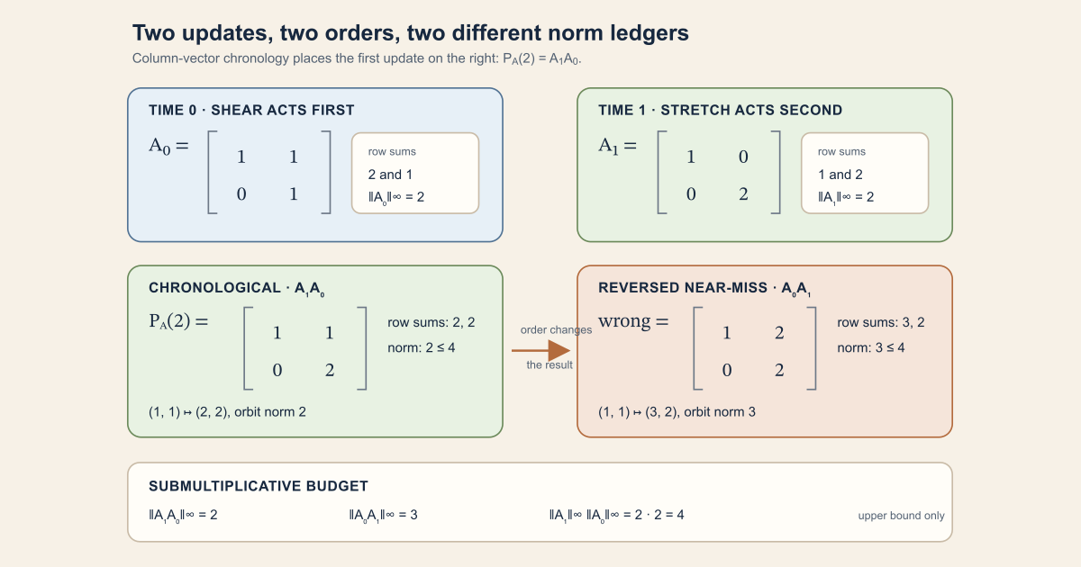
Begin with two updates that do not commute
Let a column state evolve by \(x_{j+1}=A_jx_j\). At time zero, apply the shear
\[ A_0= \begin{bmatrix} 1&1\\ 0&1 \end{bmatrix}. \]At time one, apply the anisotropic stretch
\[ A_1= \begin{bmatrix} 1&0\\ 0&2 \end{bmatrix}. \]The first map touches the vector first, so it is written on the right of the two-step product:
\[ \begin{aligned} P_A(2) &=A_1A_0\\ &= \begin{bmatrix} 1&0\\ 0&2 \end{bmatrix} \begin{bmatrix} 1&1\\ 0&1 \end{bmatrix}\\ &= \begin{bmatrix} 1&1\\ 0&2 \end{bmatrix}. \end{aligned} \]Multiplying in the tempting visual order gives something else:
\[ \begin{aligned} A_0A_1 &= \begin{bmatrix} 1&1\\ 0&1 \end{bmatrix} \begin{bmatrix} 1&0\\ 0&2 \end{bmatrix}\\ &= \begin{bmatrix} 1&2\\ 0&2 \end{bmatrix}. \end{aligned} \]The upper-right entries differ, \(1\ne2\). Thus \(A_1A_0\ne A_0A_1\): these factors do not commute. A commuting family would hide the time-order decision, so it would be a poor teaching example.
Compute the induced infinity operator norm row by row
For the norm scope used by the Lean module, a two-by-two matrix \(B=(b_{ij})\) has maximum absolute row-sum norm
\[ \lVert B\rVert_\infty {} = \max\bigl\{|b_{00}|+|b_{01}|,\ |b_{10}|+|b_{11}|\bigr\}. \]The two factor ledgers are
\[ \lVert A_0\rVert_\infty=\max\{2,1\}=2, \qquad \lVert A_1\rVert_\infty=\max\{1,2\}=2. \]The two multiplication orders have different norm ledgers:
\[ \lVert A_1A_0\rVert_\infty=\max\{2,2\}=2, \]whereas
\[ \lVert A_0A_1\rVert_\infty=\max\{3,2\}=3. \]Both satisfy submultiplicativity,
\[ \lVert A_1A_0\rVert_\infty \leq \lVert A_1\rVert_\infty\lVert A_0\rVert_\infty =4, \]and the same inequality happens to hold for the reversed product. The theorem is an upper budget, not an equality. It cannot repair a product written in the wrong order.
Let one vector expose the action order
Choose \(x=(1,1)^{\mathsf T}\), whose supremum norm is one. The chronological history gives
\[ A_1(A_0x) {} = A_1 \begin{bmatrix} 2\\ 1 \end{bmatrix} {} = \begin{bmatrix} 2\\ 2 \end{bmatrix}, \qquad \lVert A_1A_0x\rVert_\infty=2. \]Reversing the actions gives
\[ A_0(A_1x) {} = A_0 \begin{bmatrix} 1\\ 2 \end{bmatrix} {} = \begin{bmatrix} 3\\ 2 \end{bmatrix}, \qquad \lVert A_0A_1x\rVert_\infty=3. \]The finite orbit theorem permits the looser bound \(4\lVert x\rVert_\infty=4\). It does not claim that every vector attains the matrix budget.
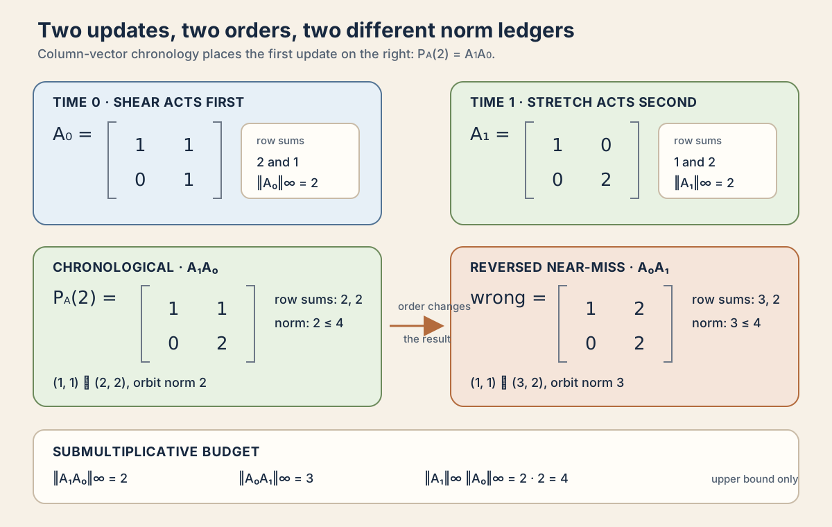
Two controlled near-misses: order and normalization
The first near-miss is now visible: writing \(A_0A_1\) because zero comes before one on the page changes the matrix, its norm, and the orbit. Matrix action is composed from right to left.
The second near-miss appears when one summarizes finite logarithmic growth. Because the chronological product in this example has positive norm, we may form the finite diagnostic
\[ g_2 {} = \frac1{2}\log\lVert P_A(2)\rVert_\infty {} = \frac12\log 2. \]The denominator is two because horizon two contains two updates. Dividing by the last factor index instead gives
\[ \widehat g_2 {} = \frac1{2-1}\log\lVert P_A(2)\rVert_\infty {} = \log2, \]which doubles the answer and already breaks at horizon one by dividing by zero. Reversing the factors creates a different finite quantity,
\[ \widetilde g_2=\frac12\log3. \]These three expressions are not Lyapunov exponents. They are calculations at one fixed horizon. The primary module defines no logarithm, no limit, no random law, and no invariant splitting. Its bound \(\lVert P_A(2)\rVert_\infty\leq2^2\) only yields, for this positive example, \(g_2\leq\log2\).
Keep six mathematical levels separate
| Level | Exact object | Present in the primary module? |
|---|---|---|
| Factor history | \(A:\mathbb N\to M_\iota(\mathbb K)\) | Yes, as a deterministic input |
| Ordered finite product | \(P_A(k)=A_{k-1}\cdots A_0\) | Yes, forwardProduct |
| Induced-norm upper bound | \(\lVert P_A(k)\rVert_\infty\leq\prod_{j\lt k}\lVert A_j\rVert_\infty\) | Yes, in positive dimension |
| Finite normalized log | \(k^{-1}\log\lVert P_A(k)\rVert_\infty\) when meaningful | No definition or theorem here |
| Random finite product and its law | \(\omega\mapsto P_{A(\omega)}(k)\) and its pushforward | Successor MeasurableFiniteProducts.lean, not this module |
| Asymptotic Lyapunov data | a limit, exponent, or invariant splitting under extra hypotheses | Not supplied by either finite-product module |
The namespace records the project’s direction; it does not make a deterministic factor sequence random. Likewise, writing one normalized logarithm does not prove its limit exists.
This chapter develops the complete public interface of
NonlinearDynamics.Random.MatrixProducts.FiniteProducts. The
module contains one definition and twelve theorems, for thirteen public
declarations in total. Nine belong to a norm-free algebraic layer. Four belong
to a positive-dimensional analytic layer. Ordered products still make sense
when the coordinate type is empty; the selected matrix norm needs a nonempty
coordinate type to normalize the identity to norm one.
Choose a route up
| Route | Begin with | Destination |
|---|---|---|
| First encounter | Begin with two updates | Multiply both orders and inspect the orbit |
| Near-miss route | Order and normalization | Separate factor order, factor count, and finite log growth |
| Algebra route | Split one history into two blocks | Understand the shifted concatenation law |
| Norm route | The vector and matrix norms | Derive the maximum-row-sum formula and action inequality |
| Lean route | Seven exact bridges | Translate chronology and bounds token by token |
| Hands-on route | Run the worksheet | Recheck every integer entry and norm locally |
| Interface route | The complete declaration map | Audit all thirteen public declarations and every assumption |
| Dynamics route | Why this finite layer matters | See how transition matrices, derivatives, and random products motivate later work |
| Boundary route | What has and has not been proved | Separate finite upper bounds from stability and ergodic conclusions |
Learning objectives
By the summit, you should be able to reproduce the opening matrix, norm, orbit, and finite-log ledgers; expand horizons zero through three without reversing time; prove the shifted split formula; distinguish algebraic from positive-dimensional analytic assumptions; read seven Lean bridges and their literal commands; and explain why a deterministic finite upper bound is not a random law, a logarithmic-growth limit, or a Lyapunov exponent.
In Lean: seven bridges from recursion to finite growth
The local worksheet later in the chapter checks the integer example with
Std. The interfaces below are the exact Mathlib-backed project
layer and use full project checks.
Bridge one: an empty history acts as the identity
MatrixProducts.forwardProduct_zero A : MatrixProducts.forwardProduct A 0 = 1MatrixProductsis the namespace containing the finite-product interface.Ais a natural-time family of square matrices.0is a horizon, meaning a factor count, not a matrix index.1is the multiplicative identity matrix at the inferred coordinate and scalar types.- The theorem is algebraic and permits an empty finite coordinate type.
The identity convention makes the zero-step action \(P_A(0)x=x\) and gives the right base case for splitting and norm induction.
Bridge two: the newest factor is prepended on the left
MatrixProducts.forwardProduct_succ A k : MatrixProducts.forwardProduct A (k + 1) = A k * MatrixProducts.forwardProduct A kk + 1is the new factor count.A kis the newest factor, whose time index isk.*is matrix multiplication.- The new factor appears on the left because column-vector actions compose from right to left.
- At
k = 1, simplification givesforwardProduct A 2 = A 1 * A 0, the opening example’s order.
Bridge three: split a history without restarting its clock
MatrixProducts.forwardProduct_add A m km + kis the total number of factors.fun j ↦ A (m + j)is the later family, reindexed so its local time zero means global timem.forwardProduct … kbuilds exactly the later block.- The early block
forwardProduct A mis on the right because it acts first. - The theorem needs associativity, not commutativity, norms, probability, or positive dimension.
Bridge four: one-step norm budgets multiply
MatrixProducts.linfty_opNorm_forwardProduct_le_prod A k- The imported scope
Matrix.Norms.Operatormakes‖A j‖the maximum absolute row-sum norm. Finset.range kcontains exactly0, …, k - 1.∏ j ∈ Finset.range k, …is a commutative product of real norm values, even though the underlying matrices do not commute.≤records an upper bound; the opening values \(2\leq4\) show that equality need not hold.- This analytic theorem assumes
[RCLike 𝕜] [Nonempty ι].
Bridge five: a uniform budget becomes a finite power
MatrixProducts.linfty_opNorm_forwardProduct_le_pow A C k hAhAis the proof of∀ j < k, ‖A j‖ ≤ C.- The strict prefix
j < kmatches the exact factors occurring in the product. C ^ kis a finite real power, not an exponential-growth limit.- The theorem does not assume stationarity or that the same matrix repeats.
- For the running example,
C = 2andk = 2give the valid budget four.
Bridge six: matrix control transfers to every vector
MatrixProducts.linfty_opNorm_forwardProduct_mulVec_le_pow A C k hA x*ᵥin the theorem conclusion is matrix-vector multiplication.xis arbitrary; no unit-norm or random-distribution assumption is present.Matrix.linfty_opNorm_mulVecsupplies the one-matrix action inequality.- The finite product theorem supplies the factor
C ^ k. - This is one-sided control. It supplies no lower expansion rate, contraction classification, or invariant direction.
Bridge seven: a finite normalized logarithm is only an expression here
Real.log ‖MatrixProducts.forwardProduct A k‖ / (k : ℝ)Real.logis Mathlib’s real logarithm, not a declaration fromFiniteProducts.lean.(k : ℝ)coerces the natural factor count into a real divisor.- The displayed mathematical interpretation explicitly requires positive horizon and norm. Lean’s arithmetic functions are total outside that domain, but totalized syntax must not be narrated as a classical growth rate there.
- No project name binds this expression in the primary module.
- No
Tendsto, probability measure, almost-everywhere quantifier, or Lyapunov-exponent theorem follows from merely typing it.
Try the exact deterministic finite-product interfaces
Full project check: pinned project plus Mathlib. Place this probe in a temporary project scratch file:
import NonlinearDynamics.Random.MatrixProducts.FiniteProducts

open scoped BigOperators Matrix Matrix.Norms.Operator
open NonlinearDynamics.Random

#print MatrixProducts.forwardProduct
#check MatrixProducts.forwardProduct_zero
#check MatrixProducts.forwardProduct_succ
#check MatrixProducts.forwardProduct_add
#check MatrixProducts.forwardProduct_one
#check MatrixProducts.forwardProduct_const
#check MatrixProducts.forwardProduct_const_one
#check MatrixProducts.forwardProduct_mulVec_zero
#check MatrixProducts.forwardProduct_mulVec_succ
#check MatrixProducts.linfty_opNorm_forwardProduct_le_prod
#check MatrixProducts.linfty_opNorm_forwardProduct_le_pow
#check MatrixProducts.linfty_opNorm_forwardProduct_mulVec_le_prod
#check MatrixProducts.linfty_opNorm_forwardProduct_mulVec_le_pow
This list is the complete thirteen-declaration public interface. #print
shows the recursive orientation; each #check invokes the pinned
elaborator and displays a theorem’s exact assumptions and conclusion. The
rendered full project command below checks the authoritative source file.
cd formalization
lake env lean -DwarningAsError=true NonlinearDynamics/Random/MatrixProducts/FiniteProducts.lean
Resource note: this exact file uses the repository's
pinned Lean and Mathlib dependencies. Initial project setup can require
substantial disk space and build time. For a lightweight first step on
macOS or Linux, use the page's standalone Lean-core or Std
tutorial.
Inspect the separate measurable-law successor
Full project check: later pinned project module plus Mathlib. The successor deliberately lives in another file:
import NonlinearDynamics.Random.MatrixProducts.MeasurableFiniteProducts

open NonlinearDynamics.Random

#check MatrixProducts.sampleForwardProduct
#check MatrixProducts.sampleForwardProduct_add
#check MatrixProducts.measurable_sampleForwardProduct
#check MatrixProducts.forwardProductLaw
#check MatrixProducts.forwardProductLaw_zero
#check MatrixProducts.forwardProductLaw_one
#check MatrixProducts.forwardProductLaw_isProbabilityMeasure
#check MatrixProducts.forwardProductProbabilityLaw
#check MatrixProducts.coe_forwardProductProbabilityLaw
These declarations add outcome-dependent sample products, exact-prefix
measurability, and a proof-carrying pushforward law. They add no independence,
stationarity, logarithmic growth, Lyapunov exponent, or asymptotic theorem.
The separation prevents the deterministic forwardProduct from
silently acquiring a probability interpretation.
cd formalization
lake env lean -DwarningAsError=true NonlinearDynamics/Random/MatrixProducts/MeasurableFiniteProducts.lean
Resource note: this exact file uses the repository's
pinned Lean and Mathlib dependencies. Initial project setup can require
substantial disk space and build time. For a lightweight first step on
macOS or Linux, use the page's standalone Lean-core or Std
tutorial.
Base camp: read the first four products
Let \(A:\mathbb N\to M_{\iota}(\mathbb K)\) be a time-indexed family of square matrices. The forward product is defined by
\[ P_A(0)=I, \qquad P_A(k+1)=A_kP_A(k). \]Expanding the recursion gives
\[ \begin{aligned} P_A(0)&=I,\\ P_A(1)&=A_0,\\ P_A(2)&=A_1A_0,\\ P_A(3)&=A_2A_1A_0. \end{aligned} \]The horizon is a factor count. Horizon three uses time indices zero, one, and two. There is no factor with index three yet.
The identity at horizon zero is the unique convention that makes an empty history perform no update. It also gives a neutral element for concatenation and agrees with the zeroth power of a constant matrix.
Written order versus action order
Matrix multiplication composes actions from right to left. For a column vector \(x\),
\[ P_A(3)x=A_2\bigl(A_1(A_0x)\bigr). \]Time moves from \(A_0\) to \(A_1\) to \(A_2\). The written product lists those factors in the reverse visual order because the output of one update becomes the input of the next. This matches the familiar composition notation \(f_2\circ f_1\circ f_0\).
Changing the recursion to \(P_A(k+1)=P_A(k)A_k\) would be a coherent but different convention. It would not represent the displayed column-vector recurrence unless the factors happened to commute.
Camp one: the Lean recursion mirrors time
The definition is structurally recursive on the natural-number horizon:
def forwardProduct (A : ℕ → Matrix ι ι 𝕜) : ℕ → Matrix ι ι 𝕜
  | 0 => 1
  | k + 1 => A k * forwardProduct A k
Two simplification theorems expose the defining equations:
@[simp] theorem forwardProduct_zero
    (A : ℕ → Matrix ι ι 𝕜) :
    forwardProduct A 0 = 1

@[simp] theorem forwardProduct_succ
    (A : ℕ → Matrix ι ι 𝕜) (k : ℕ) :
    forwardProduct A (k + 1) = A k * forwardProduct A k
The equations are true by reflexivity because they are the two branches of the definition. Publishing them under stable theorem names gives downstream proofs an interface independent of how the recursive definition is unfolded.
For vector action, the module checks both the initial and successor cases:
\[ P_A(0)x=x, \qquad P_A(k+1)x=A_k\bigl(P_A(k)x\bigr). \]The successor theorem uses Mathlib’s
Matrix.mulVec_mulVec, which states that multiplying two matrices
and then acting on a vector agrees with successive matrix-vector actions
(Mathlib contributors). No coordinate expansion is
needed.
Camp two: split one history into two blocks
Choose a split time \(m\) and a later-block length \(k\). The later block does not begin with \(A_0\); it begins with \(A_m\). Introduce the shifted family
\[ A^{(m)}_j=A_{m+j}. \]The checked formula is
\[ P_A(m+k)=P_{A^{(m)}}(k)P_A(m). \]The right factor carries the state from time zero through the first \(m\) updates. The left factor then carries that intermediate state through the next \(k\) updates. Acting on \(x\) makes the chronology explicit:
\[ P_A(m+k)x =P_{A^{(m)}}(k)\bigl(P_A(m)x\bigr). \]Check the split at five steps
Take \(m=2\) and \(k=3\). The complete product is
\[ P_A(5)=A_4A_3A_2A_1A_0. \]The early block and shifted later block are
\[ P_A(2)=A_1A_0, \qquad P_{A^{(2)}}(3)=A_4A_3A_2. \]Their chronological composition is
\[ P_{A^{(2)}}(3)P_A(2) =(A_4A_3A_2)(A_1A_0) =P_A(5). \]The Lean proof inducts on \(k\). The zero case reduces to multiplication by the identity. In the successor case, the newest factor is exposed on both sides, the induction hypothesis replaces the shorter product, and matrix multiplication associativity closes the goal.
The formula resembles a cocycle law. It is only the deterministic finite-time algebra behind such a law. The module has no base dynamical system, shift map, measurable cocycle, or probability-preserving transformation.
Camp three: constant and identity sequences
If \(A_j=B\) at every time, then
\[ P_A(k)=B^k. \]The proof again uses induction. Its successor step is
\[ P_A(k+1)=BP_A(k)=BB^k=B^{k+1}. \]The Lean proof invokes the left-oriented power formula
pow_succ’, matching the recursion’s left multiplication. If every
factor is \(I\), the result specializes to \(P_A(k)=I\) at every horizon.
These theorems connect nonautonomous and autonomous linear dynamics. An autonomous discrete system \(x_{j+1}=Bx_j\) has solution \(x_k=B^kx_0\). A time-dependent system replaces the single repeated matrix by an ordered history.
Camp four: the full assumption ledger
The source begins with two assumptions shared by both layers:
variable {𝕜 ι : Type*} [Fintype ι] [DecidableEq ι]
The complete ledger is:
| Assumption or parameter | Layer | Exact job | What it does not imply |
|---|---|---|---|
ι : Type* | Both | Names row, column, and vector coordinates | No order or numerical labeling of coordinates |
Fintype ι | Both | Makes matrix multiplication and row sums finite | No positive cardinality |
DecidableEq ι | Both | Supports the finite identity matrix and coordinate decisions | No topology or measure on the index type |
𝕜 : Type* | Both | Names the scalar type | No scalar structure by itself |
Semiring 𝕜 | Algebra | Supplies zero, one, finite sums, multiplication, and associativity | No subtraction, norm, order, inverse, or completeness |
RCLike 𝕜 | Analysis | Supplies real-or-complex analytic scalar structure used by the matrix norm interface | No randomness, stationarity, or matrix invertibility |
Nonempty ι | Analysis | Ensures the selected matrix identity has norm one | No chosen coordinate appears in theorem statements |
A : ℕ → Matrix ι ι 𝕜 | Both | Provides one deterministic factor per natural time | No measurability or law on the sequence |
m : ℕ | Split law | Chooses the first block length | No assumption that the first block is positive |
k : ℕ | Both | Chooses a finite horizon or later-block length | No passage to infinite time |
C : ℝ | Power bounds | Gives one real upper envelope for factor norms through the horizon | No separate nonnegativity premise and no optimality |
x : ι → 𝕜 | Orbit bounds | Chooses a column state | No distribution or normalization of that state |
The algebraic layer accepts an empty coordinate type. It needs no
Nonempty ι, no normed scalar field, and no probability space. The
analytic layer replaces the semiring assumption by the stronger
RCLike 𝕜 interface and adds positive dimension.
Nothing in either section assumes that a factor is invertible. Nothing assumes that two factors commute. Time is indexed by natural numbers, but there is no topology, measure, or dynamics on the time index.
Camp five: the vector and matrix norms
For a finite vector \(x:\iota\to\mathbb K\), the function-space norm is the supremum norm
\[ \lVert x\rVert_\infty=\max_i|x_i|. \]Mathlib’s normed function-space construction supplies this norm (Mathlib contributors).
The module opens the scoped matrix norm
open scoped Matrix.Norms.Operator
Within that scope,
\[ \lVert A\rVert_\infty =\max_i\sum_j|A_{ij}|. \]This is the maximum absolute row-sum norm. For positive finite dimension it is the operator norm induced by the vector supremum norm:
\[ \lVert A\rVert_\infty =\sup_{x\neq0} \frac{\lVert Ax\rVert_\infty}{\lVert x\rVert_\infty}. \]The row formula follows because one output coordinate is one row acting on the input. For each \(i\),
\[ \begin{aligned} |(Ax)_i| &=\left|\sum_jA_{ij}x_j\right|\\ &\leq\sum_j|A_{ij}|\,|x_j|\\ &\leq\left(\sum_j|A_{ij}|\right)\lVert x\rVert_\infty. \end{aligned} \]Taking the largest row proves the action inequality. Aligning input signs or complex phases with a maximizing row proves optimality. Standard matrix analysis treats this as one of the basic induced norms (Horn and Johnson). Mathlib formalizes the row-sum definition, the action inequality, submultiplicativity, and equality with the continuous-linear-map operator norm (Mathlib contributors).
The norm choice is semantic
Mathlib deliberately supports several useful finite-matrix norms. The scoped norm here is not the Frobenius norm, the Euclidean spectral operator norm, or the largest single entry magnitude.
The Hermitian Frobenius geometry entry studies
\[ \lVert A\rVert_F^2=\sum_{i,j}|A_{ij}|^2, \]an entrywise Euclidean quantity. The present norm instead asks how a matrix
acts on vector supremum size. Opening Matrix.Norms.Operator is
part of the theorem’s meaning.
Camp six: positive dimension and the empty matrix boundary
When \(\iota\) is empty, there is one vector and one square matrix. Both are trivial objects, and all algebraic declarations remain meaningful. The maximum-row-sum construction takes a finite supremum over rows. With no rows, that supremum is zero. Consequently the unique identity matrix also has norm zero.
This causes no contradiction. A norm on a trivial additive space can assign zero to its only element, because that element is both zero and the identity matrix. What fails is the separate normalization law \(\lVert I\rVert=1\).
The product-norm induction starts at
\[ \lVert P_A(0)\rVert =\lVert I\rVert =1. \]The assumption Nonempty ι is the precise condition under which
Mathlib supplies that normalized identity theorem for this scoped norm. It is
an analytic interface choice, not a ban on empty matrices. An alternative
empty-dimensional estimate could be stated separately with zero on the left,
but the current public interface chooses the familiar normalized
positive-dimensional form.
Camp seven: from one-step norms to a product bound
Submultiplicativity says
\[ \lVert AB\rVert_\infty \leq \lVert A\rVert_\infty\lVert B\rVert_\infty. \]Apply it at each successor step of the forward product:
\[ \begin{aligned} \lVert P_A(k+1)\rVert_\infty &=\lVert A_kP_A(k)\rVert_\infty\\ &\leq\lVert A_k\rVert_\infty\lVert P_A(k)\rVert_\infty. \end{aligned} \]Induction gives the first analytic theorem:
\[ \lVert P_A(k)\rVert_\infty \leq \prod_{j=0}^{k-1}\lVert A_j\rVert_\infty. \]At horizon zero, the right side is the empty scalar product, hence one. At a successor horizon, the matrix factor \(A_k\) is newest and appears on the left, while its real norm enters an ordinary scalar product. Real multiplication is commutative, so the proof may place the new scalar factor at the end to match Mathlib’s finite-range product formula. The noncommutative matrix order has not been changed; taking norms has moved the estimate into commutative real arithmetic.
The inequality can be strict. Norms discard directional cancellation and keep only worst-case amplification budgets. The theorem makes no equality or sharpness claim.
Camp eight: compress a uniform bound into a power
Assume one real number \(C\) bounds every factor norm before time \(k\):
\[ \lVert A_j\rVert_\infty\leq C \quad\text{whenever }j\lt k. \]Termwise comparison of the finite scalar products gives
\[ \prod_{j=0}^{k-1}\lVert A_j\rVert_\infty \leq \prod_{j=0}^{k-1}C =C^k. \]Combining this with the product bound yields
\[ \lVert P_A(k)\rVert_\infty\leq C^k. \]Why the constant has no explicit nonnegativity assumption
The theorem takes \(C:\mathbb R\), not a nonnegative-real value, and does not ask separately for \(0\leq C\).
If \(k\) is positive, the hypothesis includes at least one inequality \(0\leq\lVert A_j\rVert\leq C\), so \(C\) is automatically nonnegative. If \(k=0\), the quantified hypothesis is empty and
\[ C^0=1 \]for every real \(C\), including a negative one. The result then reduces to the normalized identity equation. Adding \(0\leq C\) would be mathematically harmless but stronger than necessary.
Camp nine: transfer matrix bounds to every orbit
The induced norm’s defining action estimate is
\[ \lVert Bx\rVert_\infty \leq \lVert B\rVert_\infty\lVert x\rVert_\infty. \]Take \(B=P_A(k)\), then substitute either matrix-product estimate. The module checks
\[ \lVert P_A(k)x\rVert_\infty \leq \left(\prod_{j=0}^{k-1}\lVert A_j\rVert_\infty\right) \lVert x\rVert_\infty \]and, under the uniform hypothesis,
\[ \lVert P_A(k)x\rVert_\infty \leq C^k\lVert x\rVert_\infty. \]These conclusions hold for every chosen column vector. No normalization such as \(\lVert x\rVert=1\) is required. If \(x=0\), both sides vanish. At horizon zero, the result says \(\lVert x\rVert\leq\lVert x\rVert\).
Return to the opening ledger after the general bound
The abstract theorem now explains every inequality in the opening example:
\[ \begin{aligned} \lVert P_A(2)\rVert_\infty &=\left\lVert \begin{bmatrix} 1&1\\ 0&2 \end{bmatrix} \right\rVert_\infty\\ &=2\\ &\leq \lVert A_1\rVert_\infty\lVert A_0\rVert_\infty\\ &=2\cdot2=4. \end{aligned} \]For \(x=(1,1)^{\mathsf T}\), the action estimate reads
\[ 2 =\lVert P_A(2)x\rVert_\infty \leq 4\lVert x\rVert_\infty =4. \]The exact orbit norm and exact matrix norm happen to agree here, but neither general theorem promises that coincidence. The reversed product’s norm three also lies below four, which reinforces a separate lesson: satisfying a norm bound does not certify chronological correctness.
Taking logarithms in this positive example is an optional scalar post-processing step:
\[ \frac12\log\lVert P_A(2)\rVert_\infty=\frac12\log2. \]No declaration in FiniteProducts.lean performs that step.
Consequently the checked finite bound must not be cited as a theorem about
normalized logarithmic convergence.
Type the two-step ledger yourself with Lean and Std
The project module uses Mathlib’s general matrices, scoped operator norm, and
finite products. A learner can first verify the exact integer bookkeeping with
a bounded file importing only Std. Its Matrix2 record
is a teaching model, not a replacement for the project type.
Create a scratch directory outside formalization/. Save this exact
block as OrderedMatrixProductsTutorial.lean:
import Std

namespace OrderedMatrixProductsTutorial

structure Vec2 where
  x : Int
  y : Int
  deriving Repr, DecidableEq

def Vec2.linftyNorm (v : Vec2) : Nat :=
  max v.x.natAbs v.y.natAbs

structure Matrix2 where
  a00 : Int
  a01 : Int
  a10 : Int
  a11 : Int
  deriving Repr, DecidableEq

def Matrix2.one : Matrix2 :=
  { a00 := 1, a01 := 0, a10 := 0, a11 := 1 }

def Matrix2.mul (A B : Matrix2) : Matrix2 :=
  { a00 := A.a00 * B.a00 + A.a01 * B.a10
    a01 := A.a00 * B.a01 + A.a01 * B.a11
    a10 := A.a10 * B.a00 + A.a11 * B.a10
    a11 := A.a10 * B.a01 + A.a11 * B.a11 }

def Matrix2.mulVec (A : Matrix2) (v : Vec2) : Vec2 :=
  { x := A.a00 * v.x + A.a01 * v.y
    y := A.a10 * v.x + A.a11 * v.y }

def Matrix2.linftyOpNorm (A : Matrix2) : Nat :=
  max (A.a00.natAbs + A.a01.natAbs)
      (A.a10.natAbs + A.a11.natAbs)

def forwardProduct (A : Nat → Matrix2) : Nat → Matrix2
  | 0 => Matrix2.one
  | k + 1 => (A k).mul (forwardProduct A k)

def A0 : Matrix2 :=
  { a00 := 1, a01 := 1, a10 := 0, a11 := 1 }

def A1 : Matrix2 :=
  { a00 := 1, a01 := 0, a10 := 0, a11 := 2 }

def factors : Nat → Matrix2
  | 0 => A0
  | 1 => A1
  | _ => Matrix2.one

def chronological : Matrix2 := forwardProduct factors 2
def reversed : Matrix2 := A0.mul A1
def x : Vec2 := { x := 1, y := 1 }

structure FiniteLogLedger where
  normArgument : Nat
  divisor : Nat
  deriving Repr, DecidableEq

def chronologicalRate : FiniteLogLedger :=
  { normArgument := chronological.linftyOpNorm, divisor := 2 }

def reversedRate : FiniteLogLedger :=
  { normArgument := reversed.linftyOpNorm, divisor := 2 }

def lastIndexMistake : FiniteLogLedger :=
  { normArgument := chronological.linftyOpNorm, divisor := 1 }

#eval [forwardProduct factors 0,
  forwardProduct factors 1,
  forwardProduct factors 2]

#eval [chronological, reversed]

#eval [A0.linftyOpNorm, A1.linftyOpNorm,
  chronological.linftyOpNorm, reversed.linftyOpNorm,
  A0.linftyOpNorm * A1.linftyOpNorm]

#eval [chronological.mulVec x, reversed.mulVec x]
#eval [x.linftyNorm,
  (chronological.mulVec x).linftyNorm,
  (reversed.mulVec x).linftyNorm]

#eval [chronologicalRate, reversedRate, lastIndexMistake]

#eval [decide (chronological ≠ reversed),
  decide (chronological.linftyOpNorm ≤
    A0.linftyOpNorm * A1.linftyOpNorm),
  decide (reversed.linftyOpNorm ≤
    A0.linftyOpNorm * A1.linftyOpNorm)]

example : forwardProduct factors 0 = Matrix2.one := by decide
example : forwardProduct factors 1 = A0 := by decide
example : forwardProduct factors 2 = A1.mul A0 := by decide
example : chronological =
    { a00 := 1, a01 := 1, a10 := 0, a11 := 2 } := by decide
example : reversed =
    { a00 := 1, a01 := 2, a10 := 0, a11 := 2 } := by decide
example : chronological ≠ reversed := by decide
example : chronological.linftyOpNorm = 2 := by decide
example : reversed.linftyOpNorm = 3 := by decide
example : A0.linftyOpNorm * A1.linftyOpNorm = 4 := by decide
example : (chronological.mulVec x).linftyNorm = 2 := by decide
example : (reversed.mulVec x).linftyNorm = 3 := by decide
example : chronologicalRate.divisor = 2 := by decide
example : lastIndexMistake.divisor = 1 := by decide

end OrderedMatrixProductsTutorial
Open a terminal in that scratch directory and type:
source "$HOME/.elan/env"
elan run leanprover/lean4:v4.32.0 lean OrderedMatrixProductsTutorial.lean
This exact worksheet was executed successfully with Lean 4.32.0. It printed:
[{ a00 := 1, a01 := 0, a10 := 0, a11 := 1 },
 { a00 := 1, a01 := 1, a10 := 0, a11 := 1 },
 { a00 := 1, a01 := 1, a10 := 0, a11 := 2 }]
[{ a00 := 1, a01 := 1, a10 := 0, a11 := 2 }, { a00 := 1, a01 := 2, a10 := 0, a11 := 2 }]
[2, 2, 2, 3, 4]
[{ x := 2, y := 2 }, { x := 3, y := 2 }]
[1, 2, 3]
[{ normArgument := 2, divisor := 2 }, { normArgument := 3, divisor := 2 }, { normArgument := 2, divisor := 1 }]
[true, true, true]
Read those lines as follows:
- horizons zero, one, and two are the identity, \(A_0\), and \(A_1A_0\);
- chronological and reversed products differ in their upper-right entry;
- factor, product, reverse, and budget norms are \(2,2,2,3,4\);
- the same vector becomes \((2,2)\) or \((3,2)\);
- the vector norm ledger is \(1,2,3\);
- the symbolic pairs record \((\text{norm argument},\text{factor divisor})=(2,2),(3,2),(2,1)\); and
- inequality and noncommutativity checks are all true.
The FiniteLogLedger does not implement a logarithm. It verifies
the two discrete inputs that the prose later places into
\((1/k)\log\lVert P_A(k)\rVert\): the norm argument and the factor count. This
keeps the local file small and prevents a symbolic ledger from masquerading as
a theorem about real logarithms or limits.
Every example is checked by Lean’s kernel. The command loads only
the pinned compiler and Std; it does not run Lake, import Mathlib,
or compile the project.
The complete declaration map
The module publishes exactly thirteen declarations. There are no public helper definitions beyond the product itself.
Nine algebraic declarations
| Number | Declaration | Checked statement | Main assumption boundary |
|---|---|---|---|
| 1 | forwardProduct | Defines the newest-on-left product recursively, with identity at zero | Finite decidable coordinates and semiring scalars; empty coordinates allowed |
| 2 | forwardProduct_zero | forwardProduct A 0 = 1 | Same algebraic assumptions |
| 3 | forwardProduct_succ | forwardProduct A (k + 1) = A k * forwardProduct A k | Same algebraic assumptions |
| 4 | forwardProduct_add | Splits at \(m\): shifted later product times the first \(m\) factors | No commutativity, norm, or positive dimension |
| 5 | forwardProduct_one | The one-step product is A 0 | Same algebraic assumptions |
| 6 | forwardProduct_const | A constant family equals B ^ k | Same algebraic assumptions |
| 7 | forwardProduct_const_one | The identity family has identity product at every horizon | Same algebraic assumptions |
| 8 | forwardProduct_mulVec_zero | The zero-horizon product fixes every vector | Same algebraic assumptions |
| 9 | forwardProduct_mulVec_succ | Successor action applies the earlier product first, then A k | Same algebraic assumptions |
The exact nontrivial signatures are:
theorem forwardProduct_add
    (A : ℕ → Matrix ι ι 𝕜) (m k : ℕ) :
    forwardProduct A (m + k) =
      forwardProduct (fun j => A (m + j)) k * forwardProduct A m

theorem forwardProduct_mulVec_succ
    (A : ℕ → Matrix ι ι 𝕜) (k : ℕ) (x : ι → 𝕜) :
    forwardProduct A (k + 1) *ᵥ x =
      A k *ᵥ (forwardProduct A k *ᵥ x)
Four analytic declarations
| Number | Declaration | Checked statement | Deliberate boundary |
|---|---|---|---|
| 10 | linfty_opNorm_forwardProduct_le_prod | Product matrix norm is at most the product of factor norms | Upper bound only; positive finite dimension |
| 11 | linfty_opNorm_forwardProduct_le_pow | A horizon-local uniform factor bound gives \(C^k\) | No explicit nonnegative \(C\); no asymptotic claim |
| 12 | linfty_opNorm_forwardProduct_mulVec_le_prod | Every vector orbit is bounded by the factor-norm product times its initial norm | No equality, lower bound, or stability classification |
| 13 | linfty_opNorm_forwardProduct_mulVec_le_pow | Every vector orbit is bounded by \(C^k\) times its initial norm | No convergence statement and no random hypotheses |
Their signatures are:
theorem linfty_opNorm_forwardProduct_le_prod
    (A : ℕ → Matrix ι ι 𝕜) (k : ℕ) :
    ‖forwardProduct A k‖ ≤ ∏ j ∈ Finset.range k, ‖A j‖

theorem linfty_opNorm_forwardProduct_le_pow
    (A : ℕ → Matrix ι ι 𝕜) (C : ℝ)
    (k : ℕ) (hA : ∀ j < k, ‖A j‖ ≤ C) :
    ‖forwardProduct A k‖ ≤ C ^ k

theorem linfty_opNorm_forwardProduct_mulVec_le_prod
    (A : ℕ → Matrix ι ι 𝕜) (k : ℕ) (x : ι → 𝕜) :
    ‖forwardProduct A k *ᵥ x‖ ≤
      (∏ j ∈ Finset.range k, ‖A j‖) * ‖x‖

theorem linfty_opNorm_forwardProduct_mulVec_le_pow
    (A : ℕ → Matrix ι ι 𝕜) (C : ℝ)
    (k : ℕ) (hA : ∀ j < k, ‖A j‖ ≤ C) (x : ι → 𝕜) :
    ‖forwardProduct A k *ᵥ x‖ ≤ C ^ k * ‖x‖
All four sit inside a section with
[RCLike 𝕜] [Nonempty ι]. The selected matrix norm comes from the
opened operator-norm scope. Reading the signature without that surrounding
scope and section would omit part of its mathematical meaning.
The proof architecture
The source is short because the interface composes well-chosen library facts.
| Goal | Proof mechanism | Essential imported fact |
|---|---|---|
| Split a product | Induction on later-block length | Associativity of matrix multiplication |
| Constant sequence is a power | Induction on the horizon | Left successor formula for powers |
| Chronological vector action | Rewrite one recursive step | Compatibility of matrix multiplication and matrix-vector action |
| Product norm bound | Induction on the horizon | Submultiplicativity of the scoped matrix norm |
| Uniform power bound | Compare finite scalar products term by term | Nonnegativity of norms and finite-product monotonicity |
| Product orbit bound | Apply the matrix-vector norm inequality, then the matrix bound | Induced operator-norm action estimate |
| Power orbit bound | Apply the same action estimate, then the power bound | Induced operator-norm action estimate |
No determinant expansion, eigenvalue calculation, singular-value theory, or coordinate-level product expansion is needed. The proof route stays at the weakest interface adequate for each theorem.
Why this finite layer matters
Transition matrices in linear dynamics
A nonautonomous linear difference equation uses \(P_A(k)\) as its transition from time zero to time \(k\). The split law is the finite transition-composition law. Bounds on transition matrices are a basic input to stability and dichotomy theory (Coppel). The current module supplies only the finite algebra and upper bounds, not a dichotomy or stability theorem.
Derivatives along nonlinear orbits
For a differentiable map \(f\), the chain rule classically produces products of derivatives along an orbit:
\[ D(f^k)(x) =Df(f^{k-1}(x))\cdots Df(x). \]This is exactly the chronological ordering formalized here. It motivates later connections to sensitivity, Lyapunov methods, and hyperbolicity. The present Lean file defines no differentiable map, derivative, chain-rule bridge, or nonlinear perturbation estimate. The displayed formula is mathematical motivation, not a theorem exported by this module.
Random matrix products
If each \(A_j\) depends measurably on an outcome or on a base-system orbit, the same finite product becomes a random matrix product or a cocycle iterate. Arnold develops this organization in random dynamical systems (Arnold). Oseledets’ multiplicative ergodic theorem then identifies asymptotic Lyapunov exponents under additional invariant-dynamical and logarithmic-integrability hypotheses (Oseledets).
None of that probability structure is present here. The namespace indicates the intended research direction, not hidden assumptions on the factors.
Common wrong turns
Writing factors in chronological visual order
For column vectors, \(A_0A_1A_2x\) applies \(A_2\) first. The correct three-step chronological product is \(A_2A_1A_0x\).
Treating the horizon as the last factor index
Horizon \(k\) contains \(k\) factors with indices \(0\) through \(k-1\). At horizon zero there are no factors.
Forgetting to shift the later block
After splitting at \(m\), the second block begins at \(A_m\), not at \(A_0\). The shifted family \(j\mapsto A_{m+j}\) is essential.
Reversing the split factors
The early block acts first and is therefore on the right. The later block is on the left.
Calling the scoped norm Frobenius
The analytic theorems use the maximum absolute row-sum operator norm. A Frobenius estimate may be true after separate comparison work, but it is not what these declarations state.
Assuming the matrix bound is exact
Submultiplicativity retains worst-case budgets and loses directional information. Product and power bounds can be strict, as the worked example shows.
Adding an unnecessary positive-dimension assumption
Only the analytic section assumes a nonempty coordinate type. The algebraic definition and its eight algebraic theorems support the empty type.
Demanding a nonnegative constant at zero time
At horizon zero, there are no factor inequalities and \(C^0=1\) for every real \(C\). At positive time, the hypotheses themselves force nonnegativity.
Reading a finite power bound as a Lyapunov exponent
A bound at each chosen finite horizon does not establish existence of an asymptotic logarithmic growth rate. It also supplies no lower estimate or invariant splitting.
Exercises from trailhead to summit
Trailhead
- Write \(P_A(k)\) explicitly for \(k=0,1,2,3,4\).
- Apply each of those products to \(x\), adding parentheses that expose action order.
- Verify
forwardProduct_onedirectly from the recursion. - For two noncommuting two-by-two matrices, compare \(A_1A_0x\) with \(A_0A_1x\).
Mid-mountain
- Check the split law for \(m=3\) and \(k=2\) by expanding all factors.
- Prove the split law by induction on \(k\). Mark the single use of associativity.
- Prove the constant-product theorem using the power convention \(B^{k+1}=BB^k\).
- Derive the maximum absolute row-sum bound from the triangle inequality.
- For a chosen real matrix, construct a supremum-norm-one sign vector that attains a maximizing row.
- Prove submultiplicativity by applying the action definition of the induced norm, then compare that argument with a direct row-sum proof.
Summit
- Reproduce the product-norm induction, including the empty scalar product at horizon zero and the commutation of real norm factors at the successor step.
- Explain precisely why
Nonempty ιis needed for identity norm one but not for matrix multiplication. - Construct an example where every factor has norm two but the two-step product has norm strictly less than four.
- Suppose \(0\leq C\lt1\). Derive on paper that the displayed orbit upper envelope tends to zero as \(k\) tends to infinity. List the extra real analysis and quantifier work required before calling this a Lean stability theorem.
- Design a future cocycle interface over a base map. State the measurability,
composition, and integrability fields that are absent from
forwardProduct. - State a derivative-product bridge for iterates of a differentiable map. Identify which chain-rule and domain-invariance hypotheses it would need.
Reproduce the chapter
The bounded Std worksheet above is a standalone tutorial for an
ordinary macOS or Linux host. The two exact modules import Mathlib and are
full project checks. From the repository root, run:
cd formalization
lake env lean NonlinearDynamics/Random/MatrixProducts/FiniteProducts.lean
lake env lean NonlinearDynamics/Random/MatrixProducts/MeasurableFiniteProducts.lean
These commands may require substantial disk space and memory. Technical success would still not complete the pending human mathematical, source, accessibility, scientific-integrity, and editorial reviews.
What has and has not been proved
| Topic | Status in this module |
|---|---|
| Deterministic forward product at every finite natural horizon | Defined |
| Identity convention at horizon zero | Checked |
| Newest-on-left successor recursion | Checked |
| Products at horizon one and for constant sequences | Checked |
| Shifted split after an arbitrary finite time | Checked |
| Chronological action on column vectors | Checked |
| Algebra for an empty finite coordinate type | Supported |
| Maximum absolute row-sum operator-norm product bound | Checked in positive finite dimension |
| Uniform finite-horizon power bound | Checked in positive finite dimension |
| Product and power bounds for every vector orbit | Checked in positive finite dimension |
| Equality or sharpness of any norm bound | Not claimed |
| Lower product or orbit growth bounds | Not claimed |
| Contraction, stability, exponential dichotomy, or hyperbolicity | Not proved |
| Convergence of products or vector orbits | Not proved |
| Infinite products | Not defined |
| Invertibility of factors or products | Not assumed |
| Eigenvalues, singular values, determinant, or spectral radius | Not used |
| Comparison with Frobenius or Euclidean spectral norms | Not proved |
| Random sample space, matrix law, measurability, or independence | Not defined |
| Stationarity, ergodicity, or invariant base dynamics | Not defined |
| Logarithmic integrability | Not stated |
| Lyapunov exponent or asymptotic growth-rate limit | Not defined or proved |
| Multiplicative ergodic theorem or invariant splitting | Not proved |
| Derivative or Jacobian product along a nonlinear orbit | Not connected |
| Bifurcation, chaos, or physical-model conclusion | Not claimed |
The finite layer is intentionally narrow. It fixes the object and the first growth estimates that later theories can reuse without inheriting unstated probability or asymptotic assumptions.
Where to continue
The forward matrix product glossary entry gives a compact guide to chronology, splitting, and constant powers. The induced infinity operator norm entry derives the maximum-row-sum formula, explains the matrix norm scope, and contrasts it with Frobenius geometry.
The next checked probability layer is now developed in Measurable Finite Random-Matrix Products and Proof-Carrying Pushforward Laws. Its companion finite random-matrix product entry gives the compact sample-map, exact-prefix-measurability, and law-level picture. For the broader probability vocabulary, read random matrix and Random Matrices from Outcomes to Spectra. Finite Product Probability Spaces and Independent Gaussian Fields explains a different meaning of finite product: a product measure that packages independent coordinates. Matrix products here are ordered and generally noncommutative; finite products of scalar probability measures are not the same construction.
For the alternative entrywise Euclidean norm used in the random-matrix branch, continue to Hermitian Frobenius geometry . Future chapters can build a measurable random cocycle above the new finite-law layer, connect derivative products to nonlinear dynamics, and then ask for long-time growth. Those bridges are not silently supplied by this finite module.
References
Mathlib contributors. Norms on finite matrices, Mathlib 4 documentation. This official source defines the maximum absolute row-sum matrix norm, proves matrix-product and matrix-vector inequalities, and identifies the norm with the induced continuous-linear-map operator norm on finite supremum-norm spaces.
Mathlib contributors.
Matrix-vector multiplication,
Mathlib 4 documentation. This official interface supplies
Matrix.mulVec_mulVec, the compatibility theorem that turns matrix
product recursion into chronological column-vector action.
Mathlib contributors. Normed structures on function spaces, Mathlib 4 documentation. This official source documents the finite function-space norm used as the vector supremum norm.
Roger A. Horn and Charles R. Johnson. Matrix Analysis, second edition, Cambridge University Press, 2013, International Standard Book Number (ISBN) 978-0-521-54823-6. Chapter 5 develops vector norms, induced matrix norms, and their finite-dimensional comparison. The Lean module fixes the maximum absolute row-sum convention explicitly.
W. A. Coppel. Dichotomies in Stability Theory, Lecture Notes in Mathematics, Springer, 1978. This monograph provides the classical transition-matrix and stability motivation. No dichotomy result is imported into the checked finite-product slice.
Ludwig Arnold. Random Dynamical Systems, Springer Monographs in Mathematics, 1998. The book organizes measurable cocycles and multiplicative ergodic theory in random dynamical systems. Those structures describe future applications, not present assumptions.
V. I. Oseledets. A multiplicative ergodic theorem. Characteristic Ljapunov exponents of dynamical systems, Transactions of the Moscow Mathematical Society 19 (1968), 197-231. This primary source supplies the historical long-time destination for random matrix products. The current finite upper bounds do not establish its hypotheses, exponents, limit, or invariant splitting.
The exact upstream Lean source audited for this chapter is Mathlib commit
81a5d257,
the revision pinned by formalization/lake-manifest.json.