Learning objectives
After this chapter, you should be able to:
- distinguish a parameter from iteration time;
- solve the fixed-point branches of one real family;
- read the project’s fixed and specified-period branch predicates;
- explain why a moving fixed-point set is not automatically a bifurcation;
- use a conjugacy-invariant classifier as a sufficient obstruction; and
- state what extra work is needed for a smooth fold or period-doubling theorem.
For a short definition, start with the bifurcation point glossary chapter. For the formal design record, read the Development Notebook.
One family, many update rules
A deterministic discrete-time system begins with one self-map \(f:X\to X\). Starting at \(x_0\), its orbit is
\[ x_0,\quad f(x_0),\quad f^2(x_0),\quad f^3(x_0),\ldots \]The natural number \(n\) is iteration time. A parameterized family adds a different index:
\[ F:P\to(X\to X),\qquad \mu\mapsto F_\mu. \]Here \(\mu\) chooses the update rule. Once \(\mu\) is fixed, \(n\) counts repeated applications of that selected rule. Moving horizontally on a bifurcation diagram changes \(\mu\); moving along an orbit changes \(n\).
In Lean, the family type is only an abbreviation:
abbrev ParameterizedFamily (P : Type u) (X : Type v) := P → X → X
This type does not assert continuity in \(\mu\), continuity in \(x\), or differentiability in either variable. Those hypotheses must appear when a theorem needs them.
Solve a quadratic family exactly
Consider
\[ F_\mu(x)=x+(\mu-x^2). \]The fixed-point equation cancels without approximation:
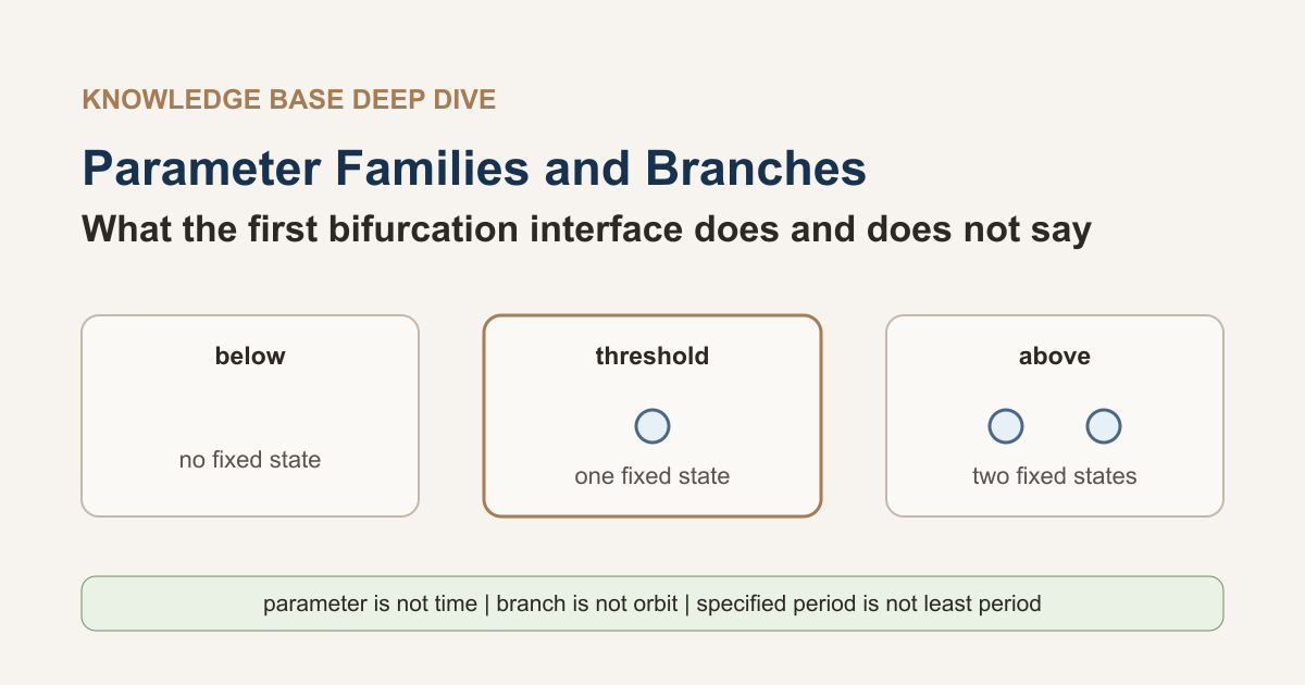
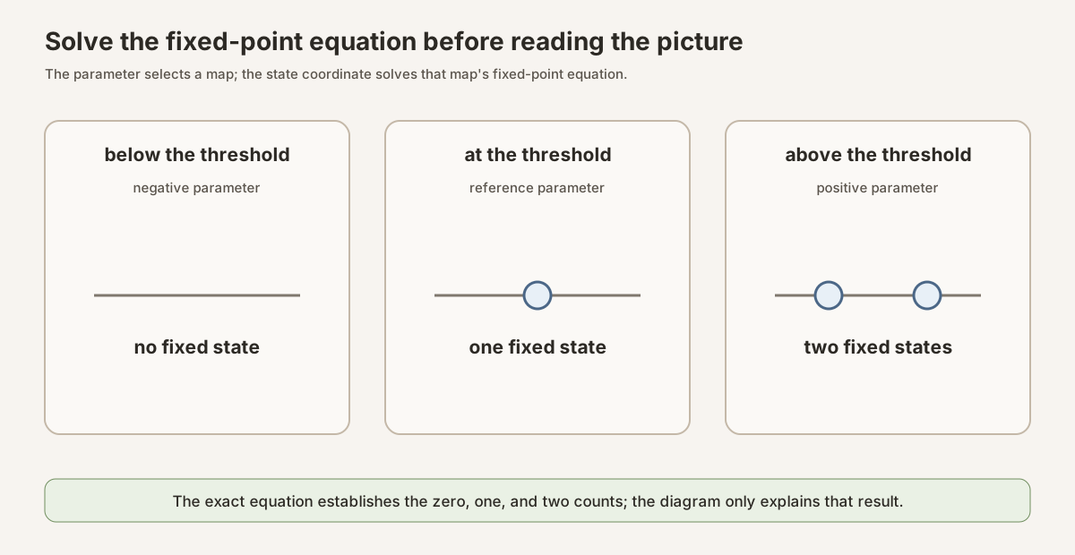
\[ F_\mu(x)=x \iff x+(\mu-x^2)=x \iff \mu=x^2. \]Because a real square is nonnegative, no real fixed point exists when \(\mu\lt0\). At \(\mu=0\), the equation forces \(x=0\). When \(\mu\gt0\), the two solutions are \(x=\sqrt\mu\) and \(x=-\sqrt\mu\).
The project source packages the cancellation as
quadraticFixedPointFamily_isFixedPt_iff. It then uses
Real.sq_sqrt to construct both square-root branches and
sq_eq_sq_iff_eq_or_eq_neg to show that these are all the fixed points for a
nonnegative parameter.
Kuznetsov analyzes \(x\mapsto\alpha+x+x^2\) and immediately notes \(x\mapsto\alpha+x-x^2\). The project family is exactly the latter after renaming \(\alpha\) to \(\mu\), as also presented in his map saddle-node article. The checked calculation here concerns the explicit family only. The generic scalar fold theorem assumes a smooth \(f(x,\alpha)\) with \(f(0,0)=0\), \(f_x(0,0)=1\), \(f_{xx}(0,0)\ne0\), and \(f_\alpha(0,0)\ne0\); those hypotheses are not bundled here.
A branch is not an orbit
A fixed-point branch chooses a fixed state for each parameter in some set \(S\):
\[ b:P\to X,\qquad F_\mu(b(\mu))=b(\mu)\quad(\mu\in S). \]The graph of \(b\) lies in parameter-state space. Its horizontal coordinate varies the map, so it is not the time evolution of one state under one map.
The project predicate is:
def IsFixedPointBranchOn (family : ParameterizedFamily P X)
    (branch : P → X) (s : Set P) : Prop :=
  ∀ μ ∈ s, Function.IsFixedPt (family μ) (branch μ)
For the quadratic family, the source proves two branches on \(S=[0,\infty)\): \(b_+(\mu)=\sqrt\mu\) and \(b_-(\mu)=-\sqrt\mu\). They coincide at zero and differ for every positive parameter.
The definition asserts only the displayed equations. It does not claim that a branch is continuous, differentiable, locally unique, maximal, stable, or attracting. Those adjectives require separate definitions and proofs.
Specified period includes fixed points
A specified-period branch for \(n\) satisfies
\[ F_\mu^n(b(\mu))=b(\mu). \]Mathlib calls this IsPeriodicPt (family μ) n (branch μ). Its convention
allows \(n=0\), and \(n\) need not be the least positive return time. A fixed
point satisfies the equation for every \(n\). More sharply, when the state
space is nonempty, the zeroth iterate is the identity, so every state satisfies
the zero-step equation and HasSpecifiedPeriodPoint f 0 cannot change.
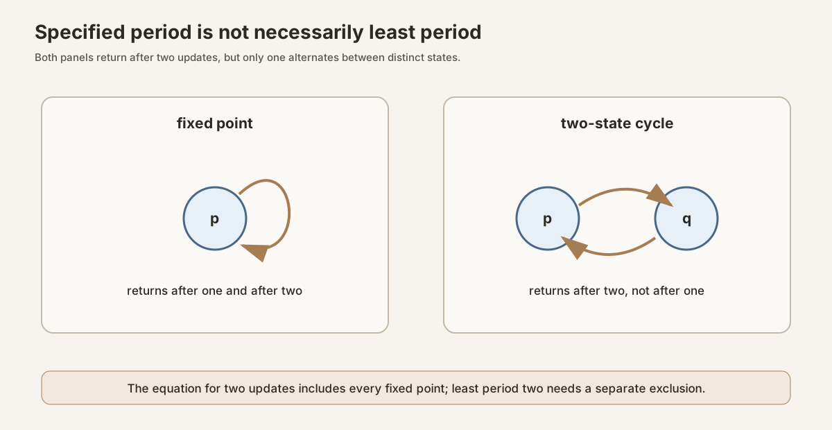
The theorem
IsFixedPointBranchOn.isSpecifiedPeriodBranchOn makes the inclusion explicit.
It applies Mathlib’s IsFixedPt.isPeriodicPt at every parameter. Therefore a
change in the existence of specified-period points must also be interpreted
carefully: for every \(n\), a fixed point already makes the classifier true.
Define qualitative equivalence before testing change
Standard bifurcation references describe a parameter where arbitrarily close systems have topologically inequivalent dynamics (Guckenheimer). The project’s first topological interface uses the already formalized conjugacy relation on the whole state space:
\[ F_\nu\sim F_\mu \]means that some homeomorphism of the entire state space intertwines the two maps. The bifurcation predicate says there is no parameter neighborhood on which every \(F_\nu\) is globally conjugate to \(F_\mu\).
This is a chosen convention. In the Lean name, Global modifies the domain of the conjugating homeomorphism. It does not classify the quadratic event as a global bifurcation in the standard local/global sense; the fold-type fixed-point event is local in that taxonomy. Local bifurcation theory often compares dynamics only near a fixed point, periodic orbit, or invariant set, so the whole-state-space relation can be stricter. Separately, this first interface does not require a continuous parameter-dependent family of conjugating homeomorphisms.
Why fixed-point-set equality gives false positives
Imagine a family in which one attracting fixed point slides from left to
right as \(\mu\) changes. The literal subsets
fixedPoints (family μ) differ because their coordinates differ. A
homeomorphism can carry the moving point at one parameter to the point at
another. The dynamics may remain conjugate.
Therefore the source does not define bifurcation as failure of local constancy of exact fixed-point sets. It uses fixed-point existence, which is invariant under conjugacy. If one map has a fixed point and a conjugate map did not, the conjugating homeomorphism would have nowhere to send that point.
Different fixed-point counts are also an obstruction when the counts are defined and compared appropriately. The first slice needs only existence, which avoids importing finite-cardinality machinery.
The classifier bridge
For any classify : P → C, the source defines a change at \(\mu\) by
¬∀ᶠ ν in 𝓝 μ, classify ν = classify μ
The notation means that no neighborhood of \(\mu\) has the reference value
everywhere. The theorem isClassificationChangeAt_iff_frequently_ne rewrites
this as different values occurring frequently in the neighborhood filter.
An arbitrary classifier may have no dynamical meaning. The generic bridge therefore asks for a proof that conjugate nearby maps have equal classifier values. The fixed-point and specified-period existence theorems supply that proof by transporting witnesses through the conjugating homeomorphism.
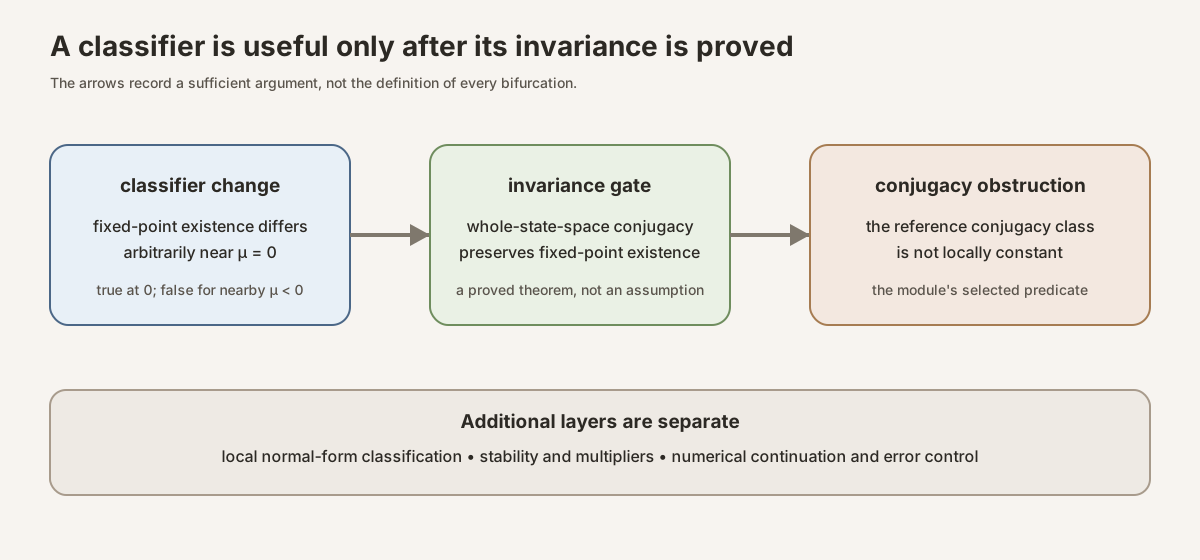
For the quadratic family at zero:
HasFixedPoint (quadraticFixedPointFamily 0)is true;- every neighborhood of zero contains a negative \(\mu\);
- the fixed-point theorem makes
HasFixedPointfalse at that \(\mu\); and - the classifier change obstructs one whole-state-space conjugacy class throughout any parameter neighborhood.
This chain establishes the module’s selected bifurcation theorem at zero. It does not claim that fixed-point existence detects every bifurcation.
A standalone finite worksheet
The file finite-branch-table.lean imports only Std. It defines three
regimes and three states. Exhaustive evaluation checks these fixed-state
lists:
| regime | fixed states |
|---|---|
below | none |
critical | center |
above | left, right |
The file also checks that the critical fixed state returns after two steps,
and that the swapped left state returns after two steps without being fixed.
Because all constructors are enumerated, by decide establishes these finite
propositions through decidable computation checked by Lean’s kernel.
Run the standalone tutorial on macOS or Linux:
elan run leanprover/lean4:v4.32.0 lean \
  site/content/knowledge-base/deep-dives/parameter-families-branches-and-bifurcation-in-discrete-time/finite-branch-table.lean
The worksheet defines no topology. If Regime is equipped with the discrete
topology, every singleton is open, so any classifier is locally constant at
each regime. The worksheet illustrates a regime ledger and the fixed/period
boundary. It does not establish a topological bifurcation in that finite
parameter space.
In Lean: the full project bridge
theorem IsFixedPointExistenceChangeAt.isGlobalTopologicalBifurcationAt\n [TopologicalSpace P] [TopologicalSpace X]\n {family : ParameterizedFamily P X} {μ : P}\n (hchange : IsFixedPointExistenceChangeAt family μ) :\n IsGlobalTopologicalBifurcationAt family μhchange is the neighborhood-level classifier change. The conclusion negates
eventual whole-state-space conjugacy. The proof uses
AreTopologicallyConjugate.hasFixedPoint_iff; it does not inspect derivatives
or a plotted branch.Try it in the repository
Create a reader worksheet containing:
import NonlinearDynamics.Deterministic.Discrete.Bifurcation

open NonlinearDynamics.Deterministic.Discrete

#check IsFixedPointExistenceChangeAt.isGlobalTopologicalBifurcationAt
#check quadraticFixedPointFamily_isGlobalTopologicalBifurcationAt_zero
import loads the checked project module. open makes this milestone’s
namespace available without repeating its full prefix. The first #check
inspects the generic fixed-point-existence bridge; the second inspects the
worked theorem at parameter zero. These commands query declarations rather
than re-proving them.
This is a full project check using pinned Lean and Mathlib dependencies. Initial setup may require substantial disk space and build time.
NonlinearDynamics/Deterministic/Discrete/Bifurcation.lean; the command below
checks the complete module with the repository’s pinned environment.cd formalization
lake env lean -DwarningAsError=true NonlinearDynamics/Deterministic/Discrete/Bifurcation.leanResource note: this exact file uses the repository's
pinned Lean and Mathlib dependencies. Initial project setup can require
substantial disk space and build time. For a lightweight first step on
macOS or Linux, use the page's standalone Lean-core or Std
tutorial.
The literal underlying command is:
cd formalization
lake env lean -DwarningAsError=true \
  NonlinearDynamics/Deterministic/Discrete/Bifurcation.lean
ParameterizedFamily is the curried type P → X → X.
∀ᶠ ν in 𝓝 μ reads “for all \(\nu\) eventually near \(\mu\).”
AreTopologicallyConjugate is the existential homeomorphism interface from
the prior milestone. propext converts a proved logical equivalence between
existence propositions into proposition equality for the generic classifier.
Lean’s elaborator constructs candidate proof terms and the kernel checks them against these formal statements. The human task remains to audit whether the chosen whole-state-space relation matches the intended mathematical question.
Misconceptions to block
| Tempting statement | What is actually established |
|---|---|
| “The branch is an orbit.” | A branch varies the parameter; an orbit varies iteration time. |
| “The fixed-point set moved, so there is a bifurcation.” | Literal set motion is coordinate-dependent. Use an equivalence relation or invariant. |
| “Return after two means period two.” | It means a specified period dividing two; fixed points are included. |
| “The count comes from the picture.” | The solved equation establishes the count; the picture explains it. |
| “A fixed-point-existence change is the definition of every bifurcation.” | It is one conjugacy-invariant sufficient witness for the selected whole-state-space predicate. |
| “This is a generic fold theorem.” | The source checks one quadratic family and does not formalize genericity hypotheses. |
| “The family is smooth because its type is parameterized.” | The type contains no regularity field. |
Exact boundary of this chapter
No theorem here supplies derivative or Jacobian criteria, multiplier crossings, hyperbolicity, implicit-function branch continuation, transversality, codimension, genericity, normal-form equivalence, stability exchange, exact least period, flip or Neimark-Sacker classification, numerical continuation, chaos, or an ODE result.
These omissions are structural. Smooth bifurcation theorems require a function-space setting, regularity, spectral conditions, and nondegeneracy assumptions. Numerical detection requires algorithms and error control. They should be layered on this interface rather than silently read into it.
References
- John Guckenheimer, “Bifurcation,” Scholarpedia 2(6):1517 (2007), DOI 10.4249/scholarpedia.1517.
- Yuri A. Kuznetsov, Elements of Applied Bifurcation Theory, 3rd ed., Applied Mathematical Sciences 112, Springer (2004), Chapters 2 and 4, DOI 10.1007/978-1-4757-3978-7.
- Yuri A. Kuznetsov, “Saddle-node bifurcation for maps,” Scholarpedia 3(4):4399 (2008), DOI 10.4249/scholarpedia.4399.
- Yuri A. Kuznetsov and Hil G. E. Meijer, Numerical Bifurcation Analysis of Maps: From Theory to Software, Cambridge University Press (2019), Chapter 2, DOI 10.1017/9781108585804. This numerical reference motivates keeping continuation and numerical error control outside the present formal interface.
- Mathlib 4.32.0 at pinned revision
81a5d257,Dynamics.FixedPoints.BasicandDynamics.PeriodicPts.Defs.