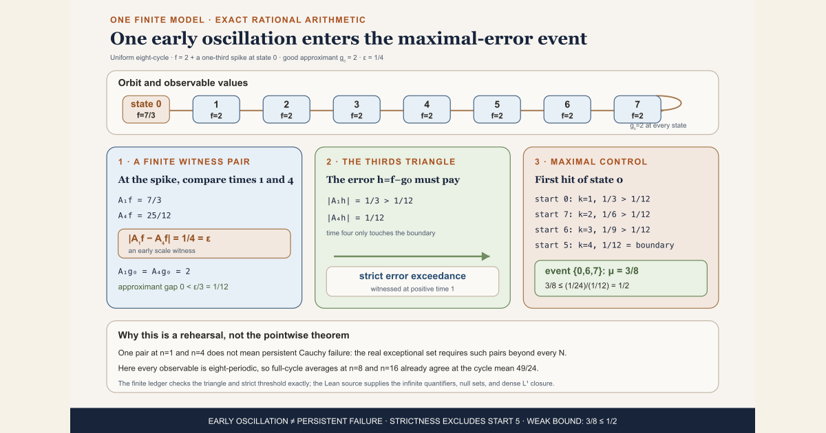
Begin with one spike on an eight-state cycle
Let
\[ \Omega=\{0,1,2,3,4,5,6,7\} \]carry the uniform probability measure, so every state has mass \(1/8\). Let \(T\) advance one place around the cycle:
\[ 0\longmapsto1\longmapsto\cdots\longmapsto7\longmapsto0. \]This transformation preserves the measure because it permutes eight equal atoms. Define the target observable \(f\) and a first approximant \(g_0\) by
\[ f(0)=2+\frac13=\frac73,\qquad f(x)=2\ \text{for }x\ne0,\qquad g_0(x)=2\ \text{for every }x. \]Thus the error \(h_0=f-g_0\) is a single spike:
\[ h_0(0)=\frac13,\qquad h_0(x)=0\ \text{for }x\ne0. \]Every observable on this finite cycle has convergent orbit averages. One complete cycle sees the same multiset of values from every start. For \(f\), the cycle sum and cycle mean are
\[ 8\cdot2+\frac13=\frac{49}{3}, \qquad \frac18\cdot\frac{49}{3}=\frac{49}{24}. \]In particular, \(A_8f(x)=A_{16}f(x)=49/24\) for all eight starts. This finite model makes pointwise goodness directly computable. Its purpose is to expose the closure arithmetic that remains valid when goodness is known only on a dense class. More explicitly, write \(n=8q+r\) with \(0\le r\lt8\). The first \(8q\) samples contribute \(q\) complete cycle sums, while the remaining prefix comes from one of finitely many bounded remainders. After division by \(n\), that remainder tends to zero and the averages tend to \(49/24\).
Compute the thirds argument at one start
Fix the Cauchy scale
\[ \varepsilon=\frac14, \qquad \frac{\varepsilon}{3}=\frac1{12}. \]Start at state \(0\), where the spike appears immediately. The target averages at times one and four are
\[ A_1f(0)=\frac73, \qquad A_4f(0) =\frac{\frac73+2+2+2}{4} =\frac{25}{12}. \]Their distance is exactly the chosen scale:
\[ \left|A_1f(0)-A_4f(0)\right| =\frac14 =\varepsilon. \]The constant approximant has no oscillation:
\[ A_1g_0(0)=A_4g_0(0)=2, \qquad \left|A_1g_0(0)-A_4g_0(0)\right| =0 \lt\frac1{12}. \]The two error averages are
\[ \left|A_1h_0(0)\right|=\frac13\gt\frac1{12}, \qquad \left|A_4h_0(0)\right|=\frac1{12}. \]The second one merely touches the boundary, while the first one strictly exceeds it. This is the concrete version of the triangle argument:
\[ \begin{aligned} \left|A_mf-A_nf\right| &\le \left|A_m(f-g)\right| +\left|A_mg-A_ng\right| +\left|A_n(f-g)\right|. \end{aligned} \]If the left side is at least \(\varepsilon\) and the middle term is strictly below \(\varepsilon/3\), the two error terms cannot both be at most \(\varepsilon/3\).
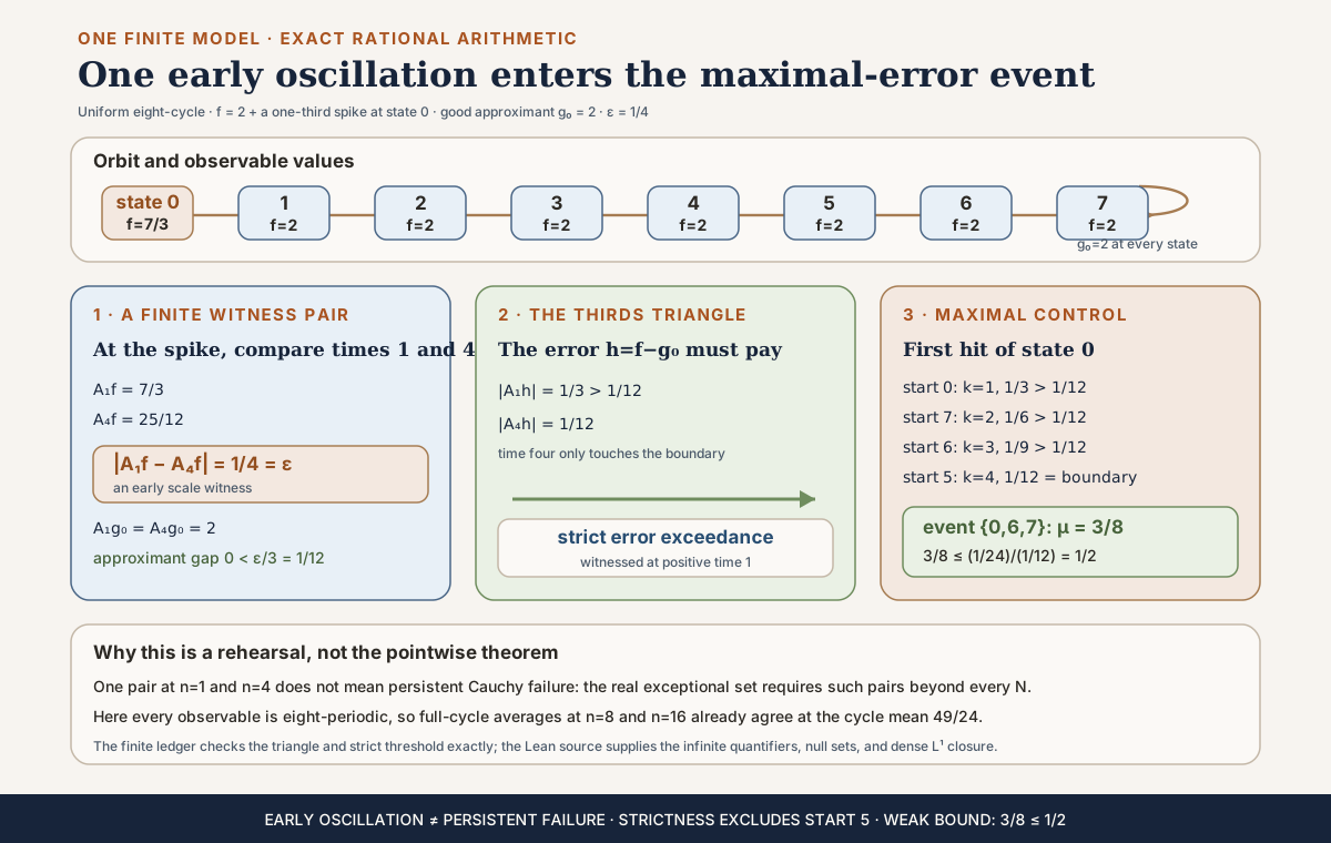
Compute the strict maximal-error event
For a start \(x\), let \(k_x\) be the first positive time at which the orbit has seen state \(0\). Before that hit, every error average is zero; at the hit, the average is \((1/3)/k_x\). Later hits cannot create a larger average. If the \(r\)-th later hit occurs at \(k_x+8r\), then
\[ \frac{(r+1)/3}{k_x+8r} \le \frac{1/3}{k_x} \]because \(k_x\le8\). Thus the first hit determines the infinite positive-time supremum in this toy system.
| start \(x\) | first-hit time \(k_x\) | largest \(|A_nh_0(x)|\) | strictly above \(1/12\)? | |—:|—:|—:|:—:| | \(0\) | \(1\) | \(1/3\) | yes | | \(1\) | \(8\) | \(1/24\) | no | | \(2\) | \(7\) | \(1/21\) | no | | \(3\) | \(6\) | \(1/18\) | no | | \(4\) | \(5\) | \(1/15\) | no | | \(5\) | \(4\) | \(1/12\) | no: equality | | \(6\) | \(3\) | \(1/9\) | yes | | \(7\) | \(2\) | \(1/6\) | yes |
Therefore the strict absolute maximal-error event is
\[ M_{1/12}(h_0)=\{0,6,7\}, \qquad \mu\bigl(M_{1/12}(h_0)\bigr)=\frac38. \]The exact \(L^1\) error is
\[ \lVert f-g_0\rVert_1 =\frac18\cdot\frac13 =\frac1{24}. \]The weak maximal estimate gives
\[ \mu\bigl(M_{1/12}(h_0)\bigr) \le \frac{\lVert h_0\rVert_1}{1/12} =\frac{1/24}{1/12} =\frac12, \]and indeed \(3/8\le1/2\).
Replace one good approximant by a dense ladder
The constant \(g_0\) is good but is not, by itself, a dense class. Use instead the dyadic-valued observables on the eight atoms. Coordinatewise dyadic approximation makes that pointwise-good family dense in this finite \(L^1\) space. To keep the ledger one-dimensional, hold the seven background values at two and vary only the spike through
\[ q_0=0,\qquad q_1=\frac14,\qquad q_2=\frac5{16},\qquad q_3=\frac{21}{64}. \]Let \(g_r\) equal \(2+q_r\) at state \(0\) and \(2\) elsewhere. Every \(g_r\) is pointwise good because it is eight-periodic. The spike heights are the successive binary truncations of \(1/3\), so
\[ \left|\frac13-q_r\right| =\frac{1}{3\cdot4^r}. \]Uniform integration and the closure estimate at \(\varepsilon=1/4\) give:
| \(r\) | spike \(q_r\) | \(\lVert f-g_r\rVert_1\) | \(3\lVert f-g_r\rVert_1/\varepsilon\) |
|---|---|---|---|
| \(0\) | \(0\) | \(1/24\) | \(1/2\) |
| \(1\) | \(1/4\) | \(1/96\) | \(1/8\) |
| \(2\) | \(5/16\) | \(1/384\) | \(1/32\) |
| \(3\) | \(21/64\) | \(1/1536\) | \(1/128\) |
The true Cauchy exceptional set \(D_{1/4}(f)\) is contained, up to the approximant’s empty bad set, in the maximal-error event for every row. Consequently,
\[ \mu\bigl(D_{1/4}(f)\bigr)\le\frac1{32} \]already at \(r=2\). A nonempty subset of this uniform finite space has mass at least \(1/8\), so \(D_{1/4}(f)\) must be empty.
That last atom-size shortcut is special to this finite model. The general Lean proof does not have a smallest positive atom. It asks for good approximants at every \(L^1\) accuracy and concludes that the exceptional measure is smaller than every positive real number, hence is zero.
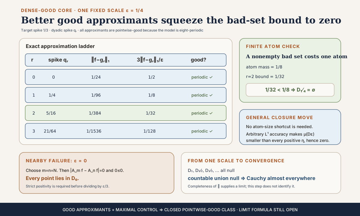
The nearby false definition
The actual exceptional event at scale \(\varepsilon\) is
\[ D_\varepsilon(f) {} = \left\{ \omega: \forall N\ \exists m,n\ge N,\ \varepsilon\le|A_mf(\omega)-A_nf(\omega)| \right\}. \]The start \(0\) has an early witness at \(m=1,n=4\), but this single pair does not put it in \(D_{1/4}(f)\). The quantifier \(\forall N\) demands new witnesses arbitrarily far out. Our periodic sequence converges, so the demand eventually fails. Replacing “beyond every \(N\)” by “for some \(m,n\)” would mistake ordinary transient motion for nonconvergence.
There is a second sharp boundary. At \(\varepsilon=0\), choose \(m=n=N\). Then
\[ 0\le|A_mf-A_nf|=0 \]for every \(N\) and every point. Hence
\[ D_0(f)=\Omega. \]This is why the quantitative closure theorems require \(0\lt\varepsilon\).
The model does not reproduce Mathlib’s \(L^p\) quotient spaces, null-set transport, or the RMT-25 fixed-plus-simple-coboundary core. It is a complete arithmetic model of their interaction: a pointwise-good approximating family, a strict maximal error event, a shrinking \(L^1\)-controlled bound, a fixed-scale Cauchy event, and the exact boundary that positivity excludes.
Writing the orbit-average formula is only the first step; its convergence requires substantial control. Begin at a state \(\omega\), apply a transformation \(T\) repeatedly, evaluate an observable \(f\) along the orbit, and average the first \(n\) readings. The resulting number is
\[ A_n f(\omega) {} = \frac{1}{n}\sum_{j=0}^{n-1}f\bigl(T^j\omega\bigr) \qquad(n\ge 1). \]The pointwise Birkhoff question asks whether the complete sequence \(A_1f(\omega),A_2f(\omega),\ldots\) converges for almost every starting state. Here almost every means that the set of exceptions has measure zero. The question is not merely whether averages converge after integration, in a norm, or along a carefully selected subsequence. It concerns every large horizon at once for nearly every individual orbit.
Random-matrix-theory milestone 26 (RMT-26) proves the following convergence form of the pointwise Birkhoff theorem in Lean:
Let \(\mu\) be a finite measure, let \(T\) preserve \(\mu\), and let \(f:\Omega\to\mathbb R\) be integrable. Then the full sequence of Birkhoff averages of \(f\) converges for \(\mu\)-almost every \(\omega\).
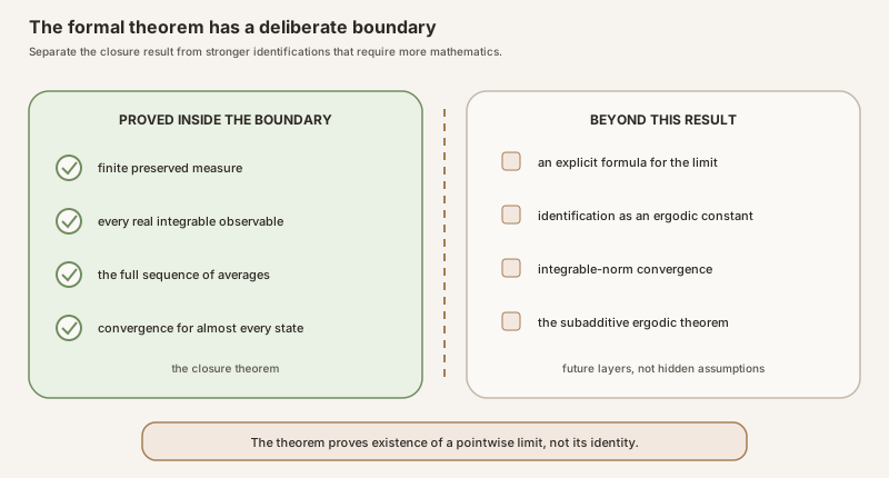
The theorem does not assume that \(\mu(\Omega)=1\). It does not assume that \(T\) is ergodic, injective, surjective, or invertible. Its conclusion is convergence-event membership. It does not identify the limit as a conditional expectation, and it does not turn the limit into a constant.
The proof joins two earlier achievements. RMT-24 supplies a weak maximal estimate that controls the set where an integrable error ever has a large positive-time average. RMT-25 supplies a dense class of square-integrable observables whose chosen representatives already have convergent averages. Finite total mass connects square integrability to ordinary integrability. The maximal estimate then makes pointwise convergence stable under \(L^1\)-approximation.
The declaration-complete implementation narrative is Finite-Measure Pointwise Birkhoff by Maximal Closure in Lean. The two main prerequisite chapters are From Finite Maximal Bounds to an Infinite Weak Estimate and Mean Is Not Pointwise: Koopman Geometry, Coboundaries, and the Missing Maximal Step. Compact definitions are available for the Birkhoff sum , Birkhoff convergence event , finite maximal ergodic inequality , and Koopman coboundary .
Choose a route up
| Route | Begin | Destination |
|---|---|---|
| Intuition | Why convergence needs stability | See the closure problem before its notation |
| Maximal route | Control absolute error averages | Convert the one-sided theorem into an absolute weak estimate |
| Cauchy route | Encode failure at one scale | Replace an unknown limit by a tail test |
| Closure route | The three-part triangle argument | Confine persistent oscillation to a maximal-error event |
| Countability route | From every scale to one conull set | Obtain full-sequence convergence |
| Density route | Why finite mass bridges L2 to L1 | Make the RMT-25 good core dense in the target space |
| Representative route | Functions and equivalence classes are different objects | Transport pointwise facts without choosing a canonical representative |
| Lean route | The checked declaration map | Match every proof stage to the public interface |
| History route | Historical lineage without anachronism | Separate Birkhoff, Yosida-Kakutani, Hopf, and Banach |
| Practice route | Solved exercises | Reconstruct the proof independently |
| Boundary route | What the theorem does not say | Avoid conditional-expectation and ergodic-constant overclaims |
Learning objectives
By the summit, a reader should be able to:
- define finite Birkhoff sums and totalized Birkhoff averages;
- state the exact finite-measure convergence theorem;
- distinguish full-sequence pointwise convergence from \(L^2\)-norm convergence;
- define a weak \((1,1)\) maximal estimate;
- prove \(|A_nh|\le A_n|h|\), including horizon zero;
- define the absolute positive-time exceedance event;
- explain why no factor two is needed in its weak estimate;
- define fixed-scale Cauchy failure with the correct inequality sidedness;
- express that event as a countable intersection and union;
- explain why representatives equal almost everywhere have equal exceptional events almost everywhere;
- derive the three-error triangle argument using \(\varepsilon/3\);
- explain why witness horizons are forced beyond zero;
- derive the quantitative fixed-scale exceptional-set bound;
- send the approximation error to zero without selecting one universal approximant;
- use reciprocal natural scales to make the conclusion countable;
- use completeness of \(\mathbb R\) to pass from Cauchy to convergence;
- define the finite-measure inclusion \(L^2\to L^1\);
- state its norm bound and interpret the zero-measure boundary;
- prove density of its range using simple functions;
- transport the RMT-25 dense good core into \(L^1\);
- track chosen representatives through the inclusion;
- audit every assumption absent from the final theorem;
- explain why convergence and limit identification are separate theorems;
- state the historically accurate roles of Birkhoff, Banach, Yosida-Kakutani, and Hopf; and
- compile and inspect the Lean interface locally.
Common setup and notation
Let \(\Omega\) be a type of states equipped with a measurable-space structure. Let \(\mu\) be a measure on \(\Omega\). A set is measurable when it belongs to the chosen sigma-algebra, the collection closed under complements and countable unions on which \(\mu\) is defined.
A map \(T:\Omega\to\Omega\) is measure preserving when it is measurable and pulling a measurable set backward through \(T\) does not change its measure. Equivalently, the pushforward of \(\mu\) by \(T\) is \(\mu\). This property lets one transport integrals and null sets along the orbit without assuming that \(T\) has an inverse.
For a real observable \(f:\Omega\to\mathbb R\), define
\[ S_n f(\omega) {} = \sum_{j=0}^{n-1}f\bigl(T^j\omega\bigr) \]and
\[ A_n f(\omega) {} = n^{-1}S_nf(\omega). \]Lean uses the inverse of the natural number after coercing it to a real. At \(n=0\), that inverse is zero and the empty sum is zero, so \(A_0f=0\). This is a totalized definition: the expression has a value at every natural horizon. Mathematical convergence concerns the tail, so changing or adding one initial term cannot affect it.
The observable \(f\) is integrable when it is almost everywhere measurable and
\[ \int_\Omega |f|\,d\mu\lt\infty. \]The corresponding norm is
\[ \lVert f\rVert_1=\int_\Omega |f|\,d\mu. \]The Lebesgue spaces \(L^1(\mu)\) and \(L^2(\mu)\) do not contain literal functions. They contain equivalence classes of functions that agree almost everywhere. Their norms are
\[ \lVert f\rVert_1=\int_\Omega |f|\,d\mu, \qquad \lVert f\rVert_2= \left(\int_\Omega |f|^2\,d\mu\right)^{1/2}. \]Lean writes these spaces as Lp ℝ 1 μ and
Lp ℝ 2 μ. The notation suppresses implementation details but
not the quotient issue. Pointwise orbit averages require actual values, so a
proof must relate each quotient vector to a chosen representative.
Why convergence needs stability
Suppose a dense class \(\mathcal G\subset L^1(\mu)\) is already known to be pointwise good: for every \(g\in\mathcal G\), the sequence \(A_ng(\omega)\) converges for almost every \(\omega\). Given arbitrary \(f\in L^1\), choose \(g\) close to \(f\). Linearity gives
\[ A_nf=A_ng+A_n(f-g). \]The first term converges almost everywhere. The second is an average of a small \(L^1\) error. Yet small \(L^1\) norm does not say that every pointwise value is small, and it does not say that every orbit average is small. A tiny set may carry very large values. The missing stability statement must control the set of points where at least one error average becomes large.
That is precisely the job of a weak maximal estimate. It does not bound the integral of the pointwise supremum. Instead, it bounds the measure of each level set of that supremum. Informally,
\[ \mu\left\{\sup_{n\ge1}|A_nh|\gt a\right\} \le \frac{\lVert h\rVert_1}{a} \qquad(a\gt0). \]The phrase weak type \((1,1)\) records this form: an \(L^1\) input norm controls the distribution tail with one inverse power of the threshold. It does not mean that the supremum itself belongs to \(L^1\).
The closure proof never needs to construct a real-valued supremum. It uses an existential event: there is some positive horizon at which the threshold is crossed. This keeps unbounded cases and extended-real choices out of the interface.
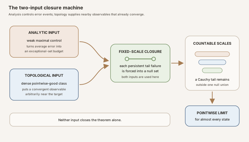
Control absolute error averages
RMT-24 proves a one-sided estimate for the event where an average of a real function rises above a threshold. RMT-26 needs absolute errors. The bridge is the elementary inequality
\[ \left|A_nh(\omega)\right| \le A_n|h|(\omega). \]For positive \(n\), expand the average and apply the triangle inequality to the finite sum:
\[ \begin{aligned} |A_nh(\omega)| &= \frac1n \left| \sum_{j=0}^{n-1}h(T^j\omega) \right|\\ &\le \frac1n \sum_{j=0}^{n-1}|h(T^j\omega)|\\ &=A_n|h|(\omega). \end{aligned} \]At \(n=0\), both sides are zero under the totalized definition. The Lean theorem therefore needs no positivity premise on \(n\):
theorem abs_birkhoffAverage_le_birkhoffAverage_abs
    (T : Ω → Ω) (f : Ω → ℝ) (n : ℕ) (ω : Ω) :
    |birkhoffAverage ℝ T f n ω| ≤
      birkhoffAverage ℝ T (fun x ↦ |f x|) n ω
For \(a\in\mathbb R\), define the absolute positive-time exceedance event
\[ M_a(h) {} = \left\{\omega: \exists k\ge1, \quad a\lt|A_kh(\omega)| \right\}. \]The event is positive-time because \(k\ge1\) is part of its definition. It is strict because RMT-24’s one-sided exceedance event is strict. The pointwise inequality immediately gives
\[ M_a(h) \subseteq \left\{\omega: \exists k\ge1, \quad a\lt A_k|h|(\omega) \right\}. \]If \(\mu\) is finite, \(T\) preserves \(\mu\), \(h\) is integrable, and \(a\gt0\), the RMT-24 theorem applied to \(|h|\) yields
\[ \mu_{\mathbb R}\bigl(M_a(h)\bigr) \le \frac{\int_\Omega |h|\,d\mu}{a}. \]Here \(\mu_{\mathbb R}(E)\) is Mathlib’s real-valued view of the extended nonnegative measure \(\mu(E)\). Finite total mass ensures that this conversion is faithful for all subsets in this module’s use. Without a finiteness fact, the conversion of infinity is totalized to zero and order reasoning can fail.
No factor two appears. One could split the two-sided event into a positive event for \(h\) and a positive event for \(-h\), but direct domination by \(A_n|h|\) is sharper and simpler. Even the split route can sum the positive and negative parts back to \(\lVert h\rVert_1\), but RMT-26 does not need that detour.
The theorem is still weak, not strong. It says how much measure can lie above each level \(a\). It does not prove
\[ \int_\Omega \sup_{n\ge1}|A_nh|\,d\mu \le C\lVert h\rVert_1. \]That strong \(L^1\) estimate is generally the wrong claim at this endpoint and is absent from the Lean file.
Encode failure at one scale
Trying to name the unknown pointwise limit too early complicates the proof. The Cauchy criterion avoids that problem. A real sequence \((x_n)\) is Cauchy when, for every \(\varepsilon\gt0\), all sufficiently late pairs are within \(\varepsilon\):
\[ \forall\varepsilon\gt0, \quad \exists N, \quad \forall m,n\ge N, \quad |x_m-x_n|\lt\varepsilon. \]Fix a scale \(\varepsilon\). RMT-26 defines the exceptional set
\[ D_\varepsilon(f) {} = \left\{\omega: \forall N, \quad \exists m,n\ge N, \quad \varepsilon\le |A_mf(\omega)-A_nf(\omega)| \right\}. \]This says that the sequence keeps making excursions of size at least \(\varepsilon\), no matter how far out one moves. Notice the non-strict inequality \(\varepsilon\le|\cdot|\). Its logical complement gives the strict tail estimate \(|\cdot|\lt\varepsilon\) required by Mathlib’s metric Cauchy criterion. Replacing it casually with a strict exceptional inequality would alter the negation and create a boundary mismatch.
The quantifiers can be displayed as a measurable countable construction:
\[ D_\varepsilon(f) {} = \bigcap_{N\in\mathbb N} \quad \bigcup_{m\ge N} \quad \bigcup_{n\ge N} \left\{\omega: \varepsilon\le|A_mf(\omega)-A_nf(\omega)| \right\}. \]When \(T\) and \(f\) are measurable, each finite average is measurable, each
comparison set is measurable, and countable unions and intersections preserve
measurability. This proves
measurableSet_birkhoffCauchyExceptionalSet.
Integrable observables are only guaranteed to be almost everywhere measurable. Lean therefore also proves a null-measurable version. A set is null measurable when it agrees with a measurable set up to a null set. That is exactly the regularity needed for measure-zero arguments involving chosen representatives.
Functions and equivalence classes are different objects
Suppose \(f=g\) almost everywhere. This does not mean that \(f(T^j\omega)=g(T^j\omega)\) for every \(\omega\). The original null set could be pulled backward along every iterate. Under quasi-measure-preserving dynamics, the preimage of a null set remains null. Taking a countable union over \(j\in\mathbb N\) still gives a null set. Outside that union, every finite orbit sample agrees, so every finite Birkhoff average agrees.
RMT-26 packages this fact at the event level:
\[ f=g\quad\text{almost everywhere} \quad\Longrightarrow\quad D_\varepsilon(f)=D_\varepsilon(g) \quad\text{almost everywhere}. \]The hypothesis used here is quasi-measure preservation, which requires
measurability and preservation of null sets but not equality of the whole
pushforward measure. The final theorem has the stronger
MeasurePreserving package, so this transport is available.
This representative bridge has two consequences. First, an almost everywhere measurable function may be replaced by its measurable representative to prove null measurability of \(D_\varepsilon(f)\). Second, an \(L^p\) quotient vector may use a chosen representative for pointwise convergence without claiming that the choice is canonical.
The distinction is logical, not cosmetic. A theorem about a quotient vector cannot be evaluated at a point until a representative is chosen. A theorem about one representative can be transported to another only after proving that orbit averages respect almost everywhere equality under the dynamics.
The three-part triangle argument
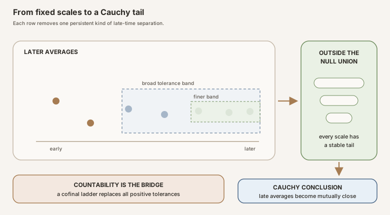
Fix \(\varepsilon\gt0\). Let \(g\) be an approximant whose Birkhoff averages converge at \(\omega\). Because convergent real sequences are Cauchy, there is a tail index \(N\) such that
\[ |A_mg(\omega)-A_ng(\omega)| \lt \frac{\varepsilon}{3} \qquad(m,n\ge N). \]Now suppose \(\omega\in D_\varepsilon(f)\). Choose the exceptional witnesses \(m,n\) beyond \(\max\{N,1\}\). The maximum with one is deliberate. It makes both horizons positive, so either one may witness the positive-time maximal event. The exceptional condition says
\[ \varepsilon \le |A_mf(\omega)-A_nf(\omega)|. \]Insert \(g\) twice and use the triangle inequality:
\[ \begin{aligned} |A_mf-A_nf| &\le |A_mf-A_mg| +|A_mg-A_ng| +|A_ng-A_nf|\\ &= |A_m(f-g)| +|A_mg-A_ng| +|A_n(f-g)|. \end{aligned} \]If neither error average strictly exceeds \(\varepsilon/3\), then both are at most \(\varepsilon/3\). The good middle term is strictly below \(\varepsilon/3\). Their sum is therefore strictly below \(\varepsilon\), contradicting the exceptional inequality. At least one error average must strictly exceed \(\varepsilon/3\).
Thus, with \(G(g)\) denoting the convergence set of \(g\),
\[ D_\varepsilon(f) \subseteq M_{\varepsilon/3}(f-g) \cup G(g)^c. \]This is an actual set inclusion. The approximant may fail on its exceptional null set, and that is why the complement \(G(g)^c\) appears explicitly. Prose that states only \(D_\varepsilon(f)\subseteq M_{\varepsilon/3}(f-g)\) has silently discarded the approximant’s bad points.
The quantitative bound
Assume \(g\) is pointwise good almost everywhere. Then \(\mu_{\mathbb R}(G(g)^c)=0\). Apply subadditivity of measure and the absolute weak maximal estimate to the inclusion:
\[ \begin{aligned} \mu_{\mathbb R}\bigl(D_\varepsilon(f)\bigr) &\le \mu_{\mathbb R}\bigl(M_{\varepsilon/3}(f-g)\bigr) +\mu_{\mathbb R}\bigl(G(g)^c\bigr)\\ &\le \frac{\int_\Omega|f-g|\,d\mu}{\varepsilon/3}. \end{aligned} \]The denominator is legal because \(\varepsilon\gt0\). The difference \(f-g\) must be integrable because the weak maximal theorem consumes an integrable error. In the final application, both \(f\) and the chosen \(L^1\) representative \(g\) are integrable, so their difference is integrable.
Send the approximation error to zero
Suppose that for every \(\delta\gt0\) there is a pointwise-good \(g\) with
\[ \int_\Omega|f-g|\,d\mu\lt\delta. \]Fix \(\eta\gt0\) and choose
\[ \delta=\eta\frac{\varepsilon}{3}. \]The quantitative bound becomes
\[ \mu_{\mathbb R}\bigl(D_\varepsilon(f)\bigr) \le \frac{\eta(\varepsilon/3)}{\varepsilon/3} =\eta. \]Because this holds for every positive \(\eta\), the nonnegative real measure of \(D_\varepsilon(f)\) is zero. Finite total mass lets Lean convert that real-measure statement back to an extended-measure nullity statement:
\[ \mu\bigl(D_\varepsilon(f)\bigr)=0. \]One does not choose a single approximant that works for every \(\eta\) or every scale. Density supplies a new approximant whenever the requested error tolerance changes. The exceptional set itself is fixed while its upper bound can be made arbitrarily small.
From every scale to one conull set
There are uncountably many positive real values of \(\varepsilon\). Measure theory closes null sets under countable unions, not arbitrary unions. The proof therefore chooses the reciprocal natural scales
\[ \varepsilon_k=\frac{1}{k+1}, \qquad k\in\mathbb N. \]Every \(\varepsilon_k\) is positive, and the sequence decreases to zero. For each \(k\), the exceptional set \(D_{\varepsilon_k}(f)\) is null. Their union
\[ N_f= \bigcup_{k\in\mathbb N}D_{1/(k+1)}(f) \]is therefore null. Take \(\omega\notin N_f\). Given any \(\varepsilon\gt0\), choose \(k\) with
\[ \frac{1}{k+1}\lt\varepsilon. \]Since \(\omega\notin D_{1/(k+1)}(f)\), the negation of the exceptional definition supplies an \(N\) such that, for all \(m,n\ge N\),
\[ |A_mf(\omega)-A_nf(\omega)| \lt \frac{1}{k+1} \lt \varepsilon. \]Thus the full sequence \(n\mapsto A_nf(\omega)\) is Cauchy. The real numbers
are complete, so the sequence converges to some real number. Lean packages
this last statement as membership in birkhoffConvergenceSet T f:
This argument proves existence of a possibly point-dependent real limit. It does not define a globally measurable limit function, and it does not say what the limit equals.
Why horizon zero causes no problem
The Cauchy exceptional witnesses may initially be any natural horizons. Inside the closure lemma they are requested beyond \(\max\{N,1\}\), so the maximal event always receives a positive witness. In the final Cauchy argument, the sequence includes \(A_0f=0\), but a finite initial prefix cannot affect convergence. The zero-horizon average is not an ordinary division by zero. It is a totalized boundary value whose information content is only that the function is defined for every natural index.
Why finite mass bridges L2 to L1
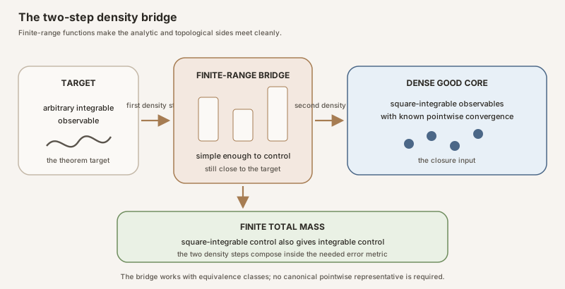
RMT-25’s dense pointwise-good class lives in real \(L^2\), while the final theorem targets real \(L^1\). On a finite measure space, Hölder’s inequality gives a continuous inclusion:
\[ \lVert h\rVert_1 \le \mu(\Omega)^{1/2}\lVert h\rVert_2. \]To see the estimate, apply the Cauchy-Schwarz inequality to \(|h|\cdot1\):
\[ \begin{aligned} \int_\Omega|h|\,d\mu &\le \left(\int_\Omega|h|^2\,d\mu\right)^{1/2} \left(\int_\Omega1^2\,d\mu\right)^{1/2}\\ &= \lVert h\rVert_2\,\mu(\Omega)^{1/2}. \end{aligned} \]The coefficient is finite precisely because the total mass is finite. RMT-26
defines first a linear map l2ToL1Linear, then bundles its
continuity as l2ToL1. In Lean’s exact real-valued coefficient,
On a probability space, \(\mu(\Omega)=1\), so the coefficient reduces to one. Probability normalization is a specialization, not an assumption of the final theorem. On the zero measure, the coefficient is zero and the operator norm is zero. Every \(L^p\) quotient then has only the zero class, so claiming that the inclusion always has norm exactly one would be false.
The inclusion is injective on equivalence classes because it retains the same underlying almost everywhere function. If two \(L^2\) classes become equal in \(L^1\), their representatives agree almost everywhere, which already makes the original \(L^2\) classes equal.
Density of the inclusion range
Continuity alone does not say that \(L^2\) is dense in \(L^1\). RMT-26 proves density using simple functions. A simple function is a measurable function with finite range. On a finite measure space, every real simple function that belongs to \(L^1\) also belongs to \(L^2\): it is essentially bounded, and finite total mass makes the integral of its squared magnitude finite.
Mathlib already proves that \(L^1\) simple functions are dense in \(L^1\).
For each such simple \(L^1\) vector, RMT-26 takes its finite-range
representative, proves it is in \(L^2\), turns it into an \(L^2\) quotient
vector, and shows that applying l2ToL1 returns the original
\(L^1\) class. Therefore the range of the inclusion contains a dense subset:
The more familiar truncation argument gives the same intuition. For \(f\in L^1\), define a bounded truncation by clipping values to \([-M,M]\). On finite measure, the clipped function is in \(L^2\), and its \(L^1\) distance from \(f\) tends to zero as \(M\to\infty\). The checked Lean proof uses the existing simple-function density API because it aligns directly with Mathlib’s quotient construction.
A dense image lemma
Let \(J:L^2\to L^1\) denote the inclusion, and let \(C\subset L^2\) be dense. If \(J\) has dense range and is continuous, then \(J(C)\) is dense in \(L^1\). To approximate a target \(f\in L^1\), first approximate it by some \(J(h)\) from the dense range. Then approximate \(h\) in \(L^2\) by \(c\in C\). Continuity makes \(J(c)\) close to \(J(h)\) in \(L^1\), and the triangle inequality completes the approximation.
RMT-26 exposes this reusable step as
dense_image_l2ToL1_of_dense. It then applies the lemma to the
RMT-25 set
fixedPlusSimpleCoboundarySetL2 hT.
That earlier core consists of sums of two kinds of quotient vectors:
- a vector fixed by the Koopman composition operator; and
- a forward Koopman coboundary generated by an \(L^2\) simple function.
Fixed representatives have constant Birkhoff averages along the orbit almost everywhere. Simple-function potentials are bounded, so their coboundary averages telescope to an endpoint difference divided by \(n\), which tends to zero. Sums preserve convergence. RMT-25 proves that this core is dense in \(L^2\) and that each member’s chosen representative is pointwise good almost everywhere.
RMT-26 defines
\[ C_1=J(C_2) \subset L^1, \]where \(C_2\) is the RMT-25 core. It proves \(C_1\) dense in \(L^1\), and it transports pointwise goodness through the almost everywhere equality between an \(L^2\) representative and the corresponding included \(L^1\) representative.
Assemble the final theorem
Let \(f:\Omega\to\mathbb R\) be integrable. Its quotient class
\(f_1\in L^1(\mu)\) is formed with hf.toL1 f. Given
\(\delta\gt0\), density of \(C_1\) supplies \(g_1\in C_1\) with
Choose the coercion of \(g_1\) back to a real function as the approximant \(g\). Its integrability is part of the \(L^1\) package. The difference \(f-g\) is integrable. Mathlib’s distance formula for real \(L^1\) gives
\[ \begin{aligned} \int_\Omega|f(\omega)-g(\omega)|\,d\mu(\omega) &= \int_\Omega \operatorname{dist}\bigl(f_1(\omega),g_1(\omega)\bigr) \,d\mu(\omega)\\ &= \operatorname{dist}_{L^1}(f_1,g_1)\\ &\lt\delta. \end{aligned} \]The first equality holds almost everywhere because the chosen representative
of hf.toL1 f agrees with \(f\) almost everywhere. Membership of
\(g_1\) in \(C_1\) supplies almost everywhere convergence of \(A_ng\).
These are exactly the three fields required by the abstract closure theorem:
- integrability of \(f-g\);
- \(L^1\) error smaller than \(\delta\); and
- almost everywhere convergence of the approximant’s averages.
The abstract theorem then yields
\[ \forall^\mu\omega, \quad \omega\in\operatorname{birkhoffConvergenceSet}(T,f), \]where \(\forall^\mu\) means “for \(\mu\)-almost every.” This is the final
declaration
ae_mem_birkhoffConvergenceSet_of_integrable.
Boundary systems are part of the theorem
The zero measure satisfies the theorem. Its almost everywhere conclusion is vacuous because every set is null, but this is a legitimate boundary case. No premise \(0\lt\mu(\Omega)\) is needed.
Identity dynamics also satisfy the theorem for every integrable observable. They are usually not ergodic unless the measure space is trivial. This probe confirms that ergodicity is absent.
A more informative probe uses Bool, the constant map sending both
states to false, and the Dirac measure concentrated at
false. The map preserves that measure but is neither injective nor
surjective. The final theorem still applies to every integrable real
observable. Thus injectivity, surjectivity, and invertibility are not hidden in
the proof.
Seven bridges from the finite ledger to Lean
The eight-cycle model computed the closure machine with rational numbers. The project module states the same moves for measurable functions, almost everywhere representatives, and arbitrarily long orbits. Each bridge below pairs a human sentence, paper mathematics, exact Lean syntax, and a token map.
Bridge 1: move the absolute value inside the orbit sum
abs_birkhoffAverage_le_birkhoffAverage_abs T f n ωTis the dynamics,fthe observable,nthe horizon, andωthe starting point.birkhoffAverage ℝfixes real-valued averages.Finset.abs_sum_le_sum_absis the finite triangle inequality underneath the theorem.- The inverse of the natural horizon is nonnegative; at horizon zero both sides are Lean’s totalized zero.
Bridge 2: turn one-sided maximal control into absolute control
measureReal_birkhoffAverageAbsoluteExceedanceSet_le hT hf hahT : MeasurePreserving T μ μsupplies the dynamical premise.hf : Integrable f μsupplies the \(L^1\) quantity \(\int|f|\,d\mu\).ha : 0 < alicenses division by the threshold.- The proof first embeds the absolute event in the one-sided event for
fun x ↦ |f x|; this is weak \((1,1)\) event control, not an \(L^1\) maximal-function norm theorem.
Bridge 3: name persistent failure at one Cauchy scale
mem_birkhoffCauchyExceptionalSet_iffbirkhoffCauchyExceptionalSet T f εis the set \(D_\varepsilon(f)\).- The outer
∀ Nis what the early \(n=1,4\) toy witness does not satisfy. - The comparison is non-strict
ε ≤ …. Its complement therefore gives the strict tail bound demanded by the metric Cauchy criterion. - At
ε = 0, choosingm = n = Nmakes every point exceptional.
Bridge 4: make the approximation error pay
birkhoffCauchyExceptionalSet_subset_exceedance_union_compl hεhε : 0 < εmakes \(\varepsilon/3\) positive.MisbirkhoffAverageAbsoluteExceedanceSet T (f - g) (ε / 3).GisbirkhoffConvergenceSet T g.- Witness horizons are chosen beyond
max N 1, so the positive-time maximal event never uses the totalized zero horizon. - The three terms in the triangle inequality are the two error averages and the approximant’s Cauchy gap.
Bridge 5: close the pointwise-good class
ae_mem_birkhoffConvergenceSet_of_dense_good hT happroxhapproxreturns an actual representativeg : Ω → ℝ, integrability off - g, a strict error-integral bound, and an almost-everywhere convergence statement.measure_birkhoffCauchyExceptionalSet_eq_zero_of_dense_goodmakes each positive fixed scale null.1 / ((k : ℝ) + 1)supplies a countable family cofinal at zero.cauchySeq_tendsto_of_completeuses completeness of \(\mathbb R\) to obtain a limit without identifying it.
Bridge 6: bring the RMT-25 good core into \(L^1\)
dense_fixedPlusSimpleCoboundarySetL1 hTl2ToL1is the continuous finite-measure inclusion on almost-everywhere equivalence classes.denseRange_l2ToL1proves its range dense using simple functions.fixedPlusSimpleCoboundarySetL1 hTis the image of the dense RMT-25 \(L^2\) core.ae_mem_birkhoffConvergenceSet_of_mem_fixedPlusSimpleCoboundarySetL1transports the chosen representative’s pointwise-good property.
Bridge 7: instantiate the closure theorem for every integrable observable
ae_mem_birkhoffConvergenceSet_of_integrable hT hf[IsFiniteMeasure μ]is a typeclass premise, not probability normalization.hf.toL1 fplaces the target in the \(L^1\) quotient space.- Density chooses a core element at every positive distance.
- The conclusion is membership in
birkhoffConvergenceSet T f. No conditional expectation or ergodic constant appears.
Type-check the exact project interface
For a full project check, place this probe in a project scratch file after installing the repository’s pinned dependencies:
import NonlinearDynamics.Random.RandomCocycles.PointwiseBirkhoff

open NonlinearDynamics.Random.RandomCocycles

#check abs_birkhoffAverage_le_birkhoffAverage_abs
#check measureReal_birkhoffAverageAbsoluteExceedanceSet_le
#check birkhoffCauchyExceptionalSet
#check birkhoffCauchyExceptionalSet_subset_exceedance_union_compl
#check measure_birkhoffCauchyExceptionalSet_eq_zero_of_dense_good
#check ae_mem_birkhoffConvergenceSet_of_dense_good
#check l2ToL1
#check dense_fixedPlusSimpleCoboundarySetL1
#check ae_mem_birkhoffConvergenceSet_of_integrable
From the repository root, type:
cd formalization
lake env lean NonlinearDynamics/Random/RandomCocycles/PointwiseBirkhoff.lean
This is a full project check. It may compile substantial dependencies and therefore may require substantial disk space and memory. It validates the authoritative 580-line module.
cd formalization
lake env lean -DwarningAsError=true NonlinearDynamics/Random/RandomCocycles/PointwiseBirkhoff.lean
Resource note: this exact file uses the repository's
pinned Lean and Mathlib dependencies. Initial project setup can require
substantial disk space and build time. For a lightweight first step on
macOS or Linux, use the page's standalone Lean-core or Std
tutorial.
Run the eight-cycle closure ledger with Std
The following file imports only Lean’s Std library. It defines the cycle,
target, dyadic approximants, exact rational averages, strict maximal event,
\(L^1\) errors, closure bounds, and the zero-scale boundary. It neither
imports Mathlib nor opens this project. Save the block byte for byte as
/tmp/PointwiseBirkhoffClosureTutorial.lean:
import Std

namespace PointwiseBirkhoffClosureTutorial

def states : List Nat :=
  List.range 8

def step (x : Nat) : Nat :=
  (x + 1) % 8

def iterate : Nat → Nat → Nat
  | 0, x => x
  | n + 1, x => iterate n (step x)

def observable (spike : Rat) (x : Nat) : Rat :=
  2 + if x % 8 = 0 then spike else 0

def orbitSum (spike : Rat) : Nat → Nat → Rat
  | 0, _ => 0
  | n + 1, x =>
      orbitSum spike n x + observable spike (iterate n x)

def average (spike : Rat) (n : Nat) (x : Nat) : Rat :=
  orbitSum spike n x / (n : Rat)

def targetSpike : Rat :=
  1 / 3

def epsilon : Rat :=
  1 / 4

def thirdsThreshold : Rat :=
  epsilon / 3

def errorAverage
    (target approximate : Rat) (n : Nat) (x : Nat) : Rat :=
  average target n x - average approximate n x

def ratAbs (q : Rat) : Rat :=
  if q < 0 then -q else q

def absoluteErrorExceedsWithinFirstCycle
    (target approximate threshold : Rat) (x : Nat) : Bool :=
  (List.range 8).any fun j =>
    decide (threshold < ratAbs
      (errorAverage target approximate (j + 1) x))

def firstCycleExceedanceStarts
    (target approximate threshold : Rat) : List Nat :=
  states.filter fun x =>
    absoluteErrorExceedsWithinFirstCycle target approximate threshold x

def uniformL1Error (target approximate : Rat) : Rat :=
  (states.foldl
    (fun total x =>
      total + ratAbs (observable target x - observable approximate x))
    0) / 8

def weakClosureBound (target approximate scale : Rat) : Rat :=
  uniformL1Error target approximate / (scale / 3)

structure TriangleLedger where
  start : Nat
  targetAverageAtOne : Rat
  targetAverageAtFour : Rat
  targetGap : Rat
  approximateAverageAtOne : Rat
  approximateAverageAtFour : Rat
  approximateGap : Rat
  oneThirdScale : Rat
  errorAverageAtOne : Rat
  errorAverageAtFour : Rat
  targetHasEarlyScaleWitness : Bool
  approximateGapIsStrictlySmall : Bool
  errorAtOneStrictlyExceeds : Bool
  errorAtFourOnlyTouchesBoundary : Bool
  deriving Repr, DecidableEq

def triangleLedger : TriangleLedger :=
  let f1 := average targetSpike 1 0
  let f4 := average targetSpike 4 0
  let g1 := average 0 1 0
  let g4 := average 0 4 0
  let e1 := errorAverage targetSpike 0 1 0
  let e4 := errorAverage targetSpike 0 4 0
  { start := 0
    targetAverageAtOne := f1
    targetAverageAtFour := f4
    targetGap := ratAbs (f1 - f4)
    approximateAverageAtOne := g1
    approximateAverageAtFour := g4
    approximateGap := ratAbs (g1 - g4)
    oneThirdScale := thirdsThreshold
    errorAverageAtOne := e1
    errorAverageAtFour := e4
    targetHasEarlyScaleWitness := decide (epsilon ≤ ratAbs (f1 - f4))
    approximateGapIsStrictlySmall :=
      decide (ratAbs (g1 - g4) < thirdsThreshold)
    errorAtOneStrictlyExceeds := decide (thirdsThreshold < ratAbs e1)
    errorAtFourOnlyTouchesBoundary :=
      decide (ratAbs e4 = thirdsThreshold) }

structure MaximalLedger where
  strictThreshold : Rat
  exceedanceStarts : List Nat
  exceedanceMeasure : Rat
  l1Error : Rat
  weakUpperBound : Rat
  weakInequalityHolds : Bool
  boundaryStart : Nat
  boundaryFirstHitTime : Nat
  boundaryErrorAverage : Rat
  boundaryIsExcludedByStrictness : Bool
  deriving Repr, DecidableEq

def maximalLedger : MaximalLedger :=
  let event :=
    firstCycleExceedanceStarts targetSpike 0 thirdsThreshold
  let eventMeasure := (event.length : Rat) / 8
  let l1 := uniformL1Error targetSpike 0
  let bound := weakClosureBound targetSpike 0 epsilon
  let boundaryAverage := errorAverage targetSpike 0 4 5
  { strictThreshold := thirdsThreshold
    exceedanceStarts := event
    exceedanceMeasure := eventMeasure
    l1Error := l1
    weakUpperBound := bound
    weakInequalityHolds := decide (eventMeasure ≤ bound)
    boundaryStart := 5
    boundaryFirstHitTime := 4
    boundaryErrorAverage := boundaryAverage
    boundaryIsExcludedByStrictness :=
      decide (¬ thirdsThreshold < ratAbs boundaryAverage) }

def dyadicApproximations : List Rat :=
  [0, 1 / 4, 5 / 16, 21 / 64]

structure ApproximationRow where
  level : Nat
  spike : Rat
  l1Error : Rat
  closureBoundAtQuarter : Rat
  averageAtEightFromZero : Rat
  averageAtSixteenFromZero : Rat
  fullCyclesAgree : Bool
  deriving Repr, DecidableEq

def approximationRow (level : Nat) (spike : Rat) : ApproximationRow :=
  let atEight := average spike 8 0
  let atSixteen := average spike 16 0
  { level := level
    spike := spike
    l1Error := uniformL1Error targetSpike spike
    closureBoundAtQuarter := weakClosureBound targetSpike spike epsilon
    averageAtEightFromZero := atEight
    averageAtSixteenFromZero := atSixteen
    fullCyclesAgree := decide (atEight = atSixteen) }

def approximationRows : List ApproximationRow :=
  (List.range dyadicApproximations.length).zipWith
    approximationRow dyadicApproximations

structure TailAndBoundaryLedger where
  targetCycleMean : Rat
  targetAveragesAtEight : List Rat
  targetAveragesAtSixteen : List Rat
  wholeCycleRowsAgree : Bool
  startZeroAveragesAtOneFourEightSixteen : List Rat
  laterWholeCyclePairAgrees : Bool
  zeroScaleSelfPairAlwaysQualifies : Bool
  atomMeasure : Rat
  thirdApproximationBound : Rat
  thirdBoundBelowOneAtom : Bool
  deriving Repr, DecidableEq

def tailAndBoundaryLedger : TailAndBoundaryLedger :=
  let atEight := states.map fun x => average targetSpike 8 x
  let atSixteen := states.map fun x => average targetSpike 16 x
  let atomMeasure : Rat := 1 / 8
  let thirdBound :=
    weakClosureBound targetSpike (5 / 16) epsilon
  { targetCycleMean := 49 / 24
    targetAveragesAtEight := atEight
    targetAveragesAtSixteen := atSixteen
    wholeCycleRowsAgree := decide (atEight = atSixteen)
    startZeroAveragesAtOneFourEightSixteen :=
      [average targetSpike 1 0, average targetSpike 4 0,
        average targetSpike 8 0, average targetSpike 16 0]
    laterWholeCyclePairAgrees :=
      decide (average targetSpike 8 0 = average targetSpike 16 0)
    zeroScaleSelfPairAlwaysQualifies :=
      decide (0 ≤ ratAbs (average targetSpike 37 3 -
        average targetSpike 37 3))
    atomMeasure := atomMeasure
    thirdApproximationBound := thirdBound
    thirdBoundBelowOneAtom := decide (thirdBound < atomMeasure) }

#eval triangleLedger
#eval maximalLedger
#eval approximationRows
#eval tailAndBoundaryLedger

example : triangleLedger.targetGap = (1 : Rat) / 4 := by
  native_decide
example : triangleLedger.approximateGap = 0 := by
  native_decide
example : triangleLedger.errorAverageAtOne = (1 : Rat) / 3 := by
  native_decide
example : triangleLedger.errorAverageAtFour = (1 : Rat) / 12 := by
  native_decide
example : triangleLedger.targetHasEarlyScaleWitness = true := by
  native_decide
example : triangleLedger.approximateGapIsStrictlySmall = true := by
  native_decide
example : triangleLedger.errorAtOneStrictlyExceeds = true := by
  native_decide
example : triangleLedger.errorAtFourOnlyTouchesBoundary = true := by
  native_decide

example : maximalLedger.exceedanceStarts = [0, 6, 7] := by
  native_decide
example : maximalLedger.exceedanceMeasure = (3 : Rat) / 8 := by
  native_decide
example : maximalLedger.l1Error = (1 : Rat) / 24 := by
  native_decide
example : maximalLedger.weakUpperBound = (1 : Rat) / 2 := by
  native_decide
example : maximalLedger.weakInequalityHolds = true := by
  native_decide
example : maximalLedger.boundaryErrorAverage = (1 : Rat) / 12 := by
  native_decide
example : maximalLedger.boundaryIsExcludedByStrictness = true := by
  native_decide

example : approximationRows.map ApproximationRow.l1Error =
    [1 / 24, 1 / 96, 1 / 384, 1 / 1536] := by
  native_decide
example : approximationRows.map ApproximationRow.closureBoundAtQuarter =
    [1 / 2, 1 / 8, 1 / 32, 1 / 128] := by
  native_decide
example : approximationRows.all ApproximationRow.fullCyclesAgree = true := by
  native_decide

example : tailAndBoundaryLedger.targetAveragesAtEight =
    List.replicate 8 (49 / 24) := by
  native_decide
example : tailAndBoundaryLedger.targetAveragesAtSixteen =
    List.replicate 8 (49 / 24) := by
  native_decide
example : tailAndBoundaryLedger.startZeroAveragesAtOneFourEightSixteen =
    [7 / 3, 25 / 12, 49 / 24, 49 / 24] := by
  native_decide
example : tailAndBoundaryLedger.zeroScaleSelfPairAlwaysQualifies = true := by
  native_decide
example : tailAndBoundaryLedger.thirdBoundBelowOneAtom = true := by
  native_decide

end PointwiseBirkhoffClosureTutorial
Important syntax:
Ratkeeps every displayed average and bound exact;List.range 8enumerates the eight starts;iterate,orbitSum, andaveragebuild the finite orbit arithmetic without Mathlib;decidecomputes a finite Boolean comparison;native_decidedischarges each finite ledger proposition with a kernel-checked decision procedure; andfirstCycleExceedanceStartsis sufficient for this single nonnegative periodic spike; the first-hit calculation above computes exactly those starts. It is not a replacement for the project’s infinite maximal-event definition.
With the pinned compiler installed, a human types:
source "$HOME/.elan/env"
elan run leanprover/lean4:v4.32.0 lean \
  /tmp/PointwiseBirkhoffClosureTutorial.lean
This is a small standalone tutorial suitable for a normal Mac or Linux
host. It imports only Std, enumerates eight states, and does not compile
Mathlib or this project. Successful execution prints exactly:
{ start := 0,
  targetAverageAtOne := (7 : Rat)/3,
  targetAverageAtFour := (25 : Rat)/12,
  targetGap := (1 : Rat)/4,
  approximateAverageAtOne := 2,
  approximateAverageAtFour := 2,
  approximateGap := 0,
  oneThirdScale := (1 : Rat)/12,
  errorAverageAtOne := (1 : Rat)/3,
  errorAverageAtFour := (1 : Rat)/12,
  targetHasEarlyScaleWitness := true,
  approximateGapIsStrictlySmall := true,
  errorAtOneStrictlyExceeds := true,
  errorAtFourOnlyTouchesBoundary := true }
{ strictThreshold := (1 : Rat)/12,
  exceedanceStarts := [0, 6, 7],
  exceedanceMeasure := (3 : Rat)/8,
  l1Error := (1 : Rat)/24,
  weakUpperBound := (1 : Rat)/2,
  weakInequalityHolds := true,
  boundaryStart := 5,
  boundaryFirstHitTime := 4,
  boundaryErrorAverage := (1 : Rat)/12,
  boundaryIsExcludedByStrictness := true }
[{ level := 0,
   spike := 0,
   l1Error := (1 : Rat)/24,
   closureBoundAtQuarter := (1 : Rat)/2,
   averageAtEightFromZero := 2,
   averageAtSixteenFromZero := 2,
   fullCyclesAgree := true },
 { level := 1,
   spike := (1 : Rat)/4,
   l1Error := (1 : Rat)/96,
   closureBoundAtQuarter := (1 : Rat)/8,
   averageAtEightFromZero := (65 : Rat)/32,
   averageAtSixteenFromZero := (65 : Rat)/32,
   fullCyclesAgree := true },
 { level := 2,
   spike := (5 : Rat)/16,
   l1Error := (1 : Rat)/384,
   closureBoundAtQuarter := (1 : Rat)/32,
   averageAtEightFromZero := (261 : Rat)/128,
   averageAtSixteenFromZero := (261 : Rat)/128,
   fullCyclesAgree := true },
 { level := 3,
   spike := (21 : Rat)/64,
   l1Error := (1 : Rat)/1536,
   closureBoundAtQuarter := (1 : Rat)/128,
   averageAtEightFromZero := (1045 : Rat)/512,
   averageAtSixteenFromZero := (1045 : Rat)/512,
   fullCyclesAgree := true }]
{ targetCycleMean := (49 : Rat)/24,
  targetAveragesAtEight := [(49 : Rat)/24,
                            (49 : Rat)/24,
                            (49 : Rat)/24,
                            (49 : Rat)/24,
                            (49 : Rat)/24,
                            (49 : Rat)/24,
                            (49 : Rat)/24,
                            (49 : Rat)/24],
  targetAveragesAtSixteen := [(49 : Rat)/24,
                              (49 : Rat)/24,
                              (49 : Rat)/24,
                              (49 : Rat)/24,
                              (49 : Rat)/24,
                              (49 : Rat)/24,
                              (49 : Rat)/24,
                              (49 : Rat)/24],
  wholeCycleRowsAgree := true,
  startZeroAveragesAtOneFourEightSixteen := [(7 : Rat)/3, (25 : Rat)/12, (49 : Rat)/24, (49 : Rat)/24],
  laterWholeCyclePairAgrees := true,
  zeroScaleSelfPairAlwaysQualifies := true,
  atomMeasure := (1 : Rat)/8,
  thirdApproximationBound := (1 : Rat)/32,
  thirdBoundBelowOneAtom := true }
The first record certifies the thirds triangle. The second certifies the strict maximal event and weak bound. The approximation rows show the closure bound shrinking by a factor of four at each level. The last record verifies the full-cycle mean, the zero-scale self-pair, and the atom-size comparison. None of these finite computations claims to formalize null sets, \(L^p\) quotients, or the infinite pointwise theorem; those are precisely the responsibilities of the project module.
The checked declaration map
The frozen 580-line RMT-26 module exposes exactly twenty-nine documented
public declarations and no private declarations. The tables preserve source
order. The SHA-256 of the audited source is
463a51c280585c932a85acab102421f70231173363fb61008c87a33f866f5253.
Layer 1: absolute maximal control
| No. | Lean declaration | Mathematical role |
|---|---|---|
| 1 | abs_birkhoffAverage_le_birkhoffAverage_abs | Proves ( |
| 2 | birkhoffAverageAbsoluteExceedanceSet | Defines the strict absolute positive-time event |
| 3 | mem_birkhoffAverageAbsoluteExceedanceSet_iff | Exposes its witness characterization |
| 4 | birkhoffAverageAbsoluteExceedanceSet_subset | Embeds it in the one-sided event for ( |
| 5 | measureReal_birkhoffAverageAbsoluteExceedanceSet_le | Gives the weak \((1,1)\) real-measure bound |
Layer 2: Cauchy failure and maximal closure
| No. | Lean declaration | Mathematical role |
|---|---|---|
| 6 | birkhoffCauchyExceptionalSet | Defines persistent non-strict failure at one scale |
| 7 | mem_birkhoffCauchyExceptionalSet_iff | Exposes the quantified tail-failure test |
| 8 | measurableSet_birkhoffCauchyExceptionalSet | Proves ordinary measurability from measurable inputs |
| 9 | birkhoffCauchyExceptionalSet_ae_eq_of_ae_eq | Transports the event across almost everywhere equal representatives |
| 10 | nullMeasurableSet_birkhoffCauchyExceptionalSet_of_aemeasurable | Handles almost everywhere measurable observables |
| 11 | nullMeasurableSet_birkhoffCauchyExceptionalSet_of_integrable | Specializes null measurability to integrable observables |
| 12 | birkhoffCauchyExceptionalSet_subset_exceedance_union_compl | Proves the three-part triangle inclusion |
| 13 | measureReal_birkhoffCauchyExceptionalSet_le | Bounds one exceptional scale by the approximation error |
| 14 | measure_birkhoffCauchyExceptionalSet_eq_zero_of_dense_good | Makes one positive scale null using arbitrarily close good approximants |
| 15 | cauchySeq_birkhoffAverage_of_not_mem_exceptional | Turns avoidance of reciprocal scales into a Cauchy sequence |
| 16 | ae_mem_birkhoffConvergenceSet_of_dense_good | States the abstract Banach-principle-style closure theorem |
The abstract closure theorem does not require integrability of \(f\) itself. Its hypotheses ask directly for integrable differences \(f-g\), arbitrarily small error integrals, and pointwise-good approximants. Integrability of the target enters later because it is the natural condition that constructs those approximants from \(L^1\).
Layer 3: the finite-measure density bridge
| No. | Lean declaration | Mathematical role |
|---|---|---|
| 17 | l2ToL1Linear | Defines the linear inclusion on quotient classes |
| 18 | l2ToL1Linear_apply_ae | Records equality of chosen representatives almost everywhere |
| 19 | norm_l2ToL1Linear_apply_le | Proves the finite-mass Hölder norm bound for each input |
| 20 | l2ToL1 | Bundles the inclusion as a continuous linear map |
| 21 | l2ToL1_apply_ae | Records representative retention for the continuous map |
| 22 | norm_l2ToL1_le | Bounds the operator norm by the square root of total mass |
| 23 | l2ToL1_injective | Proves injectivity on almost everywhere classes |
| 24 | denseRange_l2ToL1 | Proves density of the inclusion range using simple functions |
| 25 | dense_image_l2ToL1_of_dense | Sends any dense \(L^2\) set to a dense \(L^1\) image |
| 26 | fixedPlusSimpleCoboundarySetL1 | Defines the included RMT-25 core |
| 27 | dense_fixedPlusSimpleCoboundarySetL1 | Proves that core dense in \(L^1\) |
| 28 | ae_mem_birkhoffConvergenceSet_of_mem_fixedPlusSimpleCoboundarySetL1 | Retains its representative-level convergence property |
Layer 4: the final theorem
| No. | Lean declaration | Mathematical role |
|---|---|---|
| 29 | ae_mem_birkhoffConvergenceSet_of_integrable | Gives full-sequence almost everywhere convergence for every real integrable observable |
Seven anonymous compiled boundary probes
The source then checks seven propositions without adding names to the public API:
| Probe | Exact boundary checked |
|---|---|
| 1 | \(D_0(f)=\Omega\), because \(m=n=N\) witnesses \(0\le0\) |
| 2 | The \(L^2\to L^1\) operator norm is exactly zero for the zero measure |
| 3 | On a probability space, the general finite-mass norm coefficient reduces to one |
| 4 | At absolute threshold one, the weak bound has no residual division factor |
| 5 | The final theorem includes the zero-measure boundary, where its almost-everywhere conclusion is vacuous |
| 6 | Identity dynamics satisfy the final theorem for every integrable observable without ergodicity |
| 7 | A constant map on Bool preserves a Dirac mass while remaining noninjective and nonsurjective, and the final theorem still applies |
Finally, five #print axioms commands expose the axiom footprints
of:
measureReal_birkhoffAverageAbsoluteExceedanceSet_le;ae_mem_birkhoffConvergenceSet_of_dense_good;denseRange_l2ToL1;dense_fixedPlusSimpleCoboundarySetL1; andae_mem_birkhoffConvergenceSet_of_integrable.
Read the main Lean signatures
The absolute weak estimate has every analytic gate visible:
theorem measureReal_birkhoffAverageAbsoluteExceedanceSet_le
    [IsFiniteMeasure μ]
    (hT : MeasurePreserving T μ μ) (hf : Integrable f μ)
    {a : ℝ} (ha : 0 < a) :
    μ.real (birkhoffAverageAbsoluteExceedanceSet T f a) ≤
      (∫ x, |f x| ∂μ) / a
The abstract closure theorem consumes approximation data rather than a named dense subset:
theorem ae_mem_birkhoffConvergenceSet_of_dense_good
    [IsFiniteMeasure μ]
    (hT : MeasurePreserving T μ μ)
    (happrox : ∀ δ > 0, ∃ g : Ω → ℝ,
      Integrable (f - g) μ ∧
        (∫ x, |f x - g x| ∂μ) < δ ∧
          ∀ᵐ ω ∂μ, ω ∈ birkhoffConvergenceSet T g) :
    ∀ᵐ ω ∂μ, ω ∈ birkhoffConvergenceSet T f
The final theorem is intentionally short:
theorem ae_mem_birkhoffConvergenceSet_of_integrable
    [IsFiniteMeasure μ]
    (hT : MeasurePreserving T μ μ) (hf : Integrable f μ) :
    ∀ᵐ ω ∂μ, ω ∈ birkhoffConvergenceSet T f
No field for probability, ergodicity, or invertibility can be found in the signature. No limit function occurs in the conclusion.
Assumption audit
| Property | Required? | Exact role |
|---|---|---|
| Measurable space on \(\Omega\) | Yes | Supports measures, measurable observables, and almost everywhere statements |
| Finite total measure | Yes for this checked route | Makes \(L^2\to L^1\) continuous with dense range and makes real-measure conversion safe |
| Measure preservation | Yes | Supplies the maximal estimate and transports null representative differences along iterates |
| Real integrability of \(f\) | Yes in the final theorem | Places \(f\) in \(L^1\) and gives integrable approximation errors |
| Probability normalization | No | The total mass may be any finite nonnegative value |
| Positive total mass | No | The zero measure is included |
| Ergodicity | No | Convergence can hold with a nonconstant invariant limit |
| Injectivity | No | The Dirac-preserving constant-map probe compiles |
| Surjectivity | No | The same probe is nonsurjective |
| Invertibility | No | Neither direction of an inverse is used |
| Standard Borel or separability assumptions on \(\Omega\) | No | The theorem uses Mathlib’s general measurable-space interface |
Finite mass is not advertised as the sharp boundary of the pointwise ergodic theorem. It is the premise that supports this particular bridge from the RMT-25 \(L^2\) core and the RMT-24 real-measure estimate. Historically and in modern operator theory, pointwise ergodic theorems exist under broader sigma-finite or contraction settings with different proof packaging.
Historical lineage without anachronism
The modern proof combines ideas developed at different times. Treating all of them as “Birkhoff’s original proof” erases the chronology and misstates the sources.
Birkhoff in 1931
George D. Birkhoff’s 1931 paper begins with a flow generated by differential equations on a closed analytic manifold carrying invariant volume. Pages 656-657 establish an invariant-set limsup and liminf integral lemma. Pages 657-659 develop the oscillation argument, and pages 659-660 state the occupation-time result for measurable regions. This is the origin of the pointwise ergodic theorem, but it is not the exact abstract Lean interface of an arbitrary finite measure space, a possibly noninvertible endomorphism, and every real \(L^1\) observable (Birkhoff 1931).
Birkhoff could not have used Hopf’s 1954 operator theorem or the Yosida-Kakutani 1939 maximal theorem. Any sentence saying that his 1931 proof “applies Hopf’s maximal lemma” is anachronistic.
Banach in 1926
Stefan Banach’s 1926 paper predates the ergodic theorem. In the collected-work pagination, Theorem I on pages 356-359 develops continuity-in-measure control for sequences of linear operations. Theorem III on pages 359-360 gives a dense-set closure principle: under the appropriate continuity hypothesis, almost everywhere convergence on a dense subset extends to the whole Banach space (Banach 1926).
RMT-26 follows this architecture but does not invoke Banach’s theorem as a black box. Its weak maximal estimate directly supplies a quantitative continuity-at-zero argument for the relevant exceptional events. The accurate description is Banach-principle-style maximal closure.
Yosida and Kakutani in 1939
Kôsaku Yosida and Shizuo Kakutani state on page 165 that their space has a measure “of Lebesgue type,” their transformation is one-to-one and measure-preserving into the space, their observable is real and absolutely integrable, and the total measure need not be finite. Their Theorem 1 gives the Birkhoff result in Kolmogorov’s form. Their Theorem 2 is introduced as new and named the Maximal Ergodic Theorem (Yosida-Kakutani 1939).
Their theorem has broader total-measure scope but a stronger map hypothesis than RMT-26. The Lean theorem permits noninjective maps but uses finite mass in its selected density and real-measure route. Neither theorem should be called a literal restatement of the other.
Yosida’s 1940 closure proof
Yosida’s 1940 paper gives especially close historical evidence for the proof architecture. Its page 33 states a closure lemma citing Banach. Page 34 proves convergence first on a bounded dense class and extends it to the full function space. Section 3 on page 35 applies the method to an equimeasure point transformation of \((0,1)\), one-to-one almost everywhere (Yosida 1940).
RMT-26’s dense class and quantitative weak estimate differ in formal detail, but “dense good functions plus closure control” has a direct primary-source lineage.
Hopf in 1954 and Garsia in 1965
Eberhard Hopf’s 1954 paper expands the ergodic framework from transformations to positive \(L^1\) contractions and Markov operators (Hopf 1954). That operator-level generalization explains why modern texts commonly use the phrase Hopf maximal ergodic theorem. Historically careful prose should still distinguish the Yosida-Kakutani 1939 transformation theorem from Hopf’s later generalization.
Adriano Garsia’s two-page 1965 paper gives a short proof of Hopf’s maximal ergodic theorem and is the closest classical source for the finite positive-maximum peeling style used earlier in this repository (Garsia 1965).
A modern noninvertible probability formulation
Michael Keane and Karl Petersen work on a probability space with a possibly noninvertible measure-preserving transformation and \(f\in L^1\). Their main maximal theorem is on page 248, the truncation passage is on page 249, and the ergodic corollary spans pages 249-250. Their historical remarks on page 250 explicitly separate the original Birkhoff and Khinchine proofs from the later role of maximal theorems highlighted by Wiener and Yosida-Kakutani (Keane-Petersen 2006).
Their proof proceeds directly from maximal inequalities to a pointwise corollary. It does not make RMT-26’s exact \(L^2\)-core-to-\(L^1\) bridge the historical source theorem, and its probability premise is stronger than the finite-measure premise used here.
Convergence is not identification
The final theorem proves
\[ \text{for almost every }\omega, \quad \exists c_\omega\in\mathbb R, \quad A_nf(\omega)\longrightarrow c_\omega. \]Several further steps are required before one may write the usual conditional-expectation formula.
- Choose or construct a globally defined measurable representative of the pointwise limit.
- Prove that this limit is integrable. A Fatou-type bound is natural, but it is still a theorem with measurability details.
- Prove invariance under \(T\), including the endpoint-over-\(n\) argument needed for a possibly noninvertible map.
- Prove integral identities on every invariant measurable set.
- Match those identities to the defining characterization of conditional expectation onto the invariant sigma-algebra, with exact versus almost-everywhere invariance handled correctly.
- Only after adding ergodicity may one prove that the invariant limit is almost everywhere constant.
- Only after an integral identity and a positive normalization may one name that constant. On a probability space it is \(\int f\,d\mu\); on a finite space of positive mass it is \(\mu(\Omega)^{-1}\int f\,d\mu\).
The zero measure warns against dividing by total mass without a positivity premise. RMT-25’s \(L^2\) orthogonal projection identifies its norm limit in \(L^2\), but that does not automatically identify the \(L^1\) pointwise limit constructed by closure. Historically, R. V. Chacon’s separate paper titled “Identification of the Limit of Operator Averages” is itself evidence that identification is a distinct stage (Chacon 1962).
What the theorem does not say
RMT-26 proves no:
- conditional-expectation identity for the limit;
- almost everywhere constant limit;
- ergodic space-average formula;
- strong \(L^1\) bound for the maximal function;
- \(L^1\)-norm convergence of the Birkhoff averages;
- sharp infinite-measure pointwise theorem;
- canonical pointwise representative of an \(L^1\) class;
- Kingman subadditive ergodic theorem;
- samplewise random-matrix cocycle growth limit;
- Lyapunov exponent; or
- Oseledets invariant splitting.
It also does not claim that \(L^2\)-norm convergence alone implies full-sequence pointwise convergence. RMT-25 explicitly stopped at a dense pointwise-good core and, separately, an almost everywhere convergent subsequence for general \(L^2\) vectors. RMT-26 succeeds because weak maximal control makes the pointwise-good property stable under \(L^1\) approximation.
The strongest justified one-sentence conclusion is: on a finite measure-preserving system, every real integrable observable has a full sequence of Birkhoff averages that converges almost everywhere to some real limit, with no identification of that limit in this module.
Common proof failures
Failure 1: replacing weak control by norm control
The estimate bounds the measure of \(\{\exists n\ge1:|A_nh|\gt a\}\). It does not put the maximal function in \(L^1\). Integrating the level-set bound would create a logarithmic divergence at the endpoint and is not part of this proof.
Failure 2: dropping the approximant’s null set
The triangle argument works where \(g\)’s averages are Cauchy. Globally, the correct inclusion has a union with \(G(g)^c\). The complement is null, but it must be retained until measure is applied.
Failure 3: using the wrong inequality at the Cauchy boundary
The exceptional event uses \(\varepsilon\le|A_mf-A_nf|\). Its complement therefore gives a strict tail bound. Switching to a strict exceptional event without adjusting the rest of the proof loses the exact metric criterion.
Failure 4: forgetting positive witness times
The maximal event requires \(n\ge1\). Requesting Cauchy witnesses beyond \(\max\{N,1\}\) is what connects the tail event to that positive-time definition. The totalized \(A_0f=0\) is not a positive average.
Failure 5: treating an Lp class as a literal function
Point evaluation is representative-dependent. Every use of a quotient representative must be accompanied by the almost everywhere equality and the orbit transport theorem that preserves the convergence event.
Failure 6: calling finite mass necessary for every Birkhoff theorem
Finite mass is needed by this checked density bridge and real-measure route. The classical literature contains broader infinite-measure or positive- operator versions. State the scope of the formal theorem, not a false sharpness claim.
Failure 7: identifying the limit from convergence alone
Existence of \(c_\omega\) does not prove measurability, invariance, integrability, a conditional-expectation identity, or constancy. Each belongs to a later theorem.
Solved exercises
Exercise 1: calibrate the zero horizon
Show that \(A_0f(\omega)=0\) under the totalized definition and explain why this value cannot change convergence.
Solution. The range of summation is empty, so \(S_0f(\omega)=0\). The real inverse of zero is totalized to zero, hence \(A_0f(\omega)=0\cdot0=0\). Convergence depends only on sufficiently late terms. Replacing, deleting, or adding finitely many initial terms preserves convergence, so this boundary value has no effect on the theorem.
Exercise 2: prove absolute domination
Prove \(|A_nh(\omega)|\le A_n|h|(\omega)\) for every natural \(n\).
Solution. For \(n\ge1\), pull the nonnegative factor \(1/n\) outside the absolute value and apply the finite-sum triangle inequality: \(|\sum_jh(T^j\omega)|\le\sum_j|h(T^j\omega)|\). Multiplication by \(1/n\ge0\) preserves the inequality. For \(n=0\), both sides are zero, so the same theorem holds without a case-dependent public statement.
Exercise 3: derive the event inclusion
Why does \(M_a(h)\subseteq E_a(|h|)\), where \(E_a\) is the one-sided positive-time exceedance event?
Solution. A point in \(M_a(h)\) comes with a positive horizon \(k\) and the strict inequality \(a\lt|A_kh|\). Absolute domination gives \(|A_kh|\le A_k|h|\). Transitivity yields \(a\lt A_k|h|\), with the same positive witness \(k\), exactly the membership condition for \(E_a(|h|)\).
Exercise 4: explain the weak type constant
Why does the direct argument produce coefficient one rather than two?
Solution. Both signs are controlled simultaneously by the nonnegative observable \(|h|\): \(|A_nh|\le A_n|h|\). Applying the one-sided weak estimate to \(|h|\) gives numerator \(\int|h|=\lVert h\rVert_1\) once. A union bound over separate events for \(h\) and \(-h\) is unnecessary.
Exercise 5: test threshold zero for Cauchy failure
Show that \(D_0(f)=\Omega\) for every \(f\).
Solution. Given any point \(\omega\) and tail index \(N\), choose \(m=n=N\). Then \(|A_mf(\omega)-A_nf(\omega)|=0\), so the required inequality \(0\le0\) holds. Every point belongs to the exceptional set. This is why the quantitative closure theorem requires \(\varepsilon\gt0\).
Exercise 6: negate the exceptional event
Write the logical negation of \(\omega\in D_\varepsilon(f)\).
Solution. Negating “for every \(N\), there exist \(m,n\ge N\) with \(\varepsilon\le|A_mf-A_nf|\)” gives: there exists \(N\) such that for all \(m,n\ge N\), one has \(|A_mf-A_nf|\lt\varepsilon\). The strict comparison is exactly why the exceptional definition uses a non-strict inequality.
Exercise 7: prove measurability of one scale
Assume \(T\) and \(f\) are measurable. Why is \(D_\varepsilon(f)\) measurable?
Solution. Every iterate \(T^j\) is measurable, so each orbit sample and finite average is measurable. Differences and absolute values of measurable real functions are measurable. Therefore each comparison set \(\{\varepsilon\le|A_mf-A_nf|\}\) is measurable. The displayed construction of \(D_\varepsilon(f)\) uses only countable intersections and countable unions, which preserve measurability.
Exercise 8: locate the null-set transport
If \(f=g\) almost everywhere, why is measure preservation relevant to their orbit averages?
Solution. Equality may fail on a null set \(N\). At time \(j\), the orbit samples can differ only on \((T^j)^{-1}(N)\). A quasi-measure-preserving map sends null sets backward to null sets. The countable union of these preimages over all \(j\) is null. Outside it, every finite orbit sample and hence every finite average agrees for \(f\) and \(g\).
Exercise 9: reconstruct the thirds argument
Assume the middle approximant difference is strictly below \(\varepsilon/3\), while both error averages are at most \(\varepsilon/3\). What contradiction follows at an exceptional pair?
Solution. The three-part triangle inequality makes the target difference strictly less than \(\varepsilon/3+\varepsilon/3+\varepsilon/3=\varepsilon\). But an exceptional pair satisfies the opposite non-strict inequality \(\varepsilon\le|A_mf-A_nf|\). The two statements are incompatible, so at least one error average must strictly exceed \(\varepsilon/3\).
Exercise 10: explain the maximum with one
Why does the Lean proof request exceptional witnesses beyond \(\max\{N,1\}\) rather than merely beyond \(N\)?
Solution. The good approximant needs witnesses beyond its Cauchy tail index \(N\). The absolute maximal event additionally requires a positive horizon. Passing to \(\max\{N,1\}\) satisfies both conditions at once, so either witness \(m\) or \(n\) can enter the positive-time event.
Exercise 11: calculate the quantitative scale
Suppose \(\int|f-g|\,d\mu\lt\eta\varepsilon/3\). What bound follows for \(\mu_{\mathbb R}(D_\varepsilon(f))\)?
Solution. The fixed-scale closure estimate gives
\[ \mu_{\mathbb R}(D_\varepsilon(f)) \le \frac{\int|f-g|\,d\mu}{\varepsilon/3} \lt \frac{\eta(\varepsilon/3)}{\varepsilon/3} =\eta. \]Positivity of \(\varepsilon\) licenses the division.
Exercise 12: turn arbitrary bounds into zero
Why does \(0\le x\le\eta\) for every \(\eta\gt0\) imply \(x=0\)?
Solution. If \(x\gt0\), choose \(\eta=x/2\). Then \(x\le x/2\), a contradiction. Lean uses an order lemma expressing the same Archimedean fact. The closure proof applies it to the nonnegative real number \(\mu_{\mathbb R}(D_\varepsilon(f))\).
Exercise 13: justify reciprocal scales
Why are \(1/(k+1)\) sufficient even though the Cauchy criterion quantifies over every positive real \(\varepsilon\)?
Solution. For every \(\varepsilon\gt0\), the Archimedean property gives a natural \(k\) with \(1/(k+1)\lt\varepsilon\). A tail whose pairwise distances are below the smaller reciprocal threshold is automatically a tail whose distances are below \(\varepsilon\). The reciprocal family is countable and cofinal at zero.
Exercise 14: finish with completeness
What property of \(\mathbb R\) is used after all reciprocal exceptional sets are removed?
Solution. Outside their union, the Birkhoff-average sequence is Cauchy.
The real numbers form a complete metric space, meaning every Cauchy sequence
converges to a real number. This is the only step that produces the existential
limit required by birkhoffConvergenceSet.
Exercise 15: derive the finite-mass inclusion coefficient
Use Cauchy-Schwarz to find the norm coefficient of \(L^2\to L^1\).
Solution. Apply Cauchy-Schwarz to \(|h|\) and the constant function one:
\[ \begin{aligned} \lVert h\rVert_1 &\le \lVert h\rVert_2\lVert1\rVert_2\\ &= \mu(\Omega)^{1/2}\lVert h\rVert_2. \end{aligned} \]The coefficient is finite when \(\mu(\Omega)\lt\infty\).
Exercise 16: inspect the zero-measure coefficient
Why is the inclusion operator norm zero rather than one for the zero measure?
Solution. Every measurable function has \(L^1\) and \(L^2\) seminorm zero under the zero measure, so each quotient space contains only its zero vector. The unique linear map between these zero spaces has operator norm zero. The bound \(\lVert J\rVert\le\mu(\Omega)^{1/2}=0\) is exact.
Exercise 17: prove simple functions are square integrable
Let \(s\) be a real simple function on a finite measure space. Why does \(s\in L^1\) imply \(s\in L^2\)?
Solution. A finite-range real function has an essential bound \(M\). Then \(|s|^2\le M^2\) everywhere, so \(\int|s|^2\,d\mu\le M^2\mu(\Omega)\lt\infty\). Its measurability is part of being a measurable simple function. Thus it defines an \(L^2\) class.
Exercise 18: prove density of the image core
Let \(J:X\to Y\) be continuous with dense range, and let \(C\subset X\) be dense. Why is \(J(C)\) dense in \(Y\)?
Solution. Given \(y\in Y\) and tolerance \(\varepsilon\), first choose \(x\in X\) with \(Jx\) within \(\varepsilon/2\) of \(y\). Continuity at \(x\) supplies a neighborhood whose image lies within \(\varepsilon/2\) of \(Jx\). Density of \(C\) supplies \(c\) in that neighborhood. The triangle inequality makes \(Jc\) within \(\varepsilon\) of \(y\).
Exercise 19: separate the two density facts
What are the two distinct density statements used in RMT-26?
Solution. First, the RMT-25 fixed-plus-simple-coboundary set is dense in \(L^2\). Second, the finite-measure inclusion \(L^2\to L^1\) has dense range. Continuity combines them to show that the included RMT-25 core is dense in \(L^1\). Neither statement alone yields the final density conclusion.
Exercise 20: identify the final approximation distance
Why does the \(L^1\) distance between real quotient vectors equal the integral of the absolute representative difference?
Solution. In a real metric space,
\(\operatorname{dist}(x,y)=|x-y|\). Mathlib’s \(L^1\) distance theorem
integrates this pointwise distance between chosen representatives. The
representative of hf.toL1 f agrees with \(f\) almost everywhere,
so integral congruence replaces it by the original observable without changing
the integral.
Exercise 21: test identity dynamics
Compute the positive-time Birkhoff averages when \(T\) is the identity.
Solution. Every orbit sample is \(f(\omega)\), so \(S_nf(\omega)=nf(\omega)\) and \(A_nf(\omega)=f(\omega)\) for \(n\ge1\). The sequence converges immediately. This example may be highly nonergodic, confirming that ergodicity is unnecessary for convergence.
Exercise 22: test the noninjective Dirac system
Let \(S:\mathrm{Bool}\to\mathrm{Bool}\) send every input to
false, and let \(\mu\) be the Dirac measure at
false. Why does \(S\) preserve \(\mu\)?
Solution. The support point false is fixed by \(S\). Mapping
the Dirac measure through a measurable map produces the Dirac measure at the
image of its support, which is again false. The map is neither
injective nor surjective, so the final theorem’s application here rules out
both properties as hidden assumptions.
Exercise 23: distinguish convergence from an ergodic constant
Why can the final limit be nonconstant when ergodicity is absent?
Solution. Under identity dynamics, the positive-time averages equal \(f(\omega)\). Unless \(f\) is almost everywhere constant, their limit varies with \(\omega\). The theorem promises convergence, not constancy. Ergodicity is the separate rigidity property that later forces invariant integrable limits to be almost everywhere constant.
Exercise 24: state the probability specialization
What does probability normalization change in the \(L^2\to L^1\) estimate?
Solution. It sets \(\mu(\Omega)=1\), so \(\lVert h\rVert_1\le\lVert h\rVert_2\) and the inclusion operator norm is at most one. It does not change the closure logic. RMT-26 keeps the more general finite-mass coefficient and therefore needs no probability typeclass.
Exercise 25: diagnose a false historical sentence
What is wrong with “Birkhoff proved his 1931 theorem using Hopf’s maximal ergodic lemma”?
Solution. The chronology makes it impossible. Yosida and Kakutani named the transformation maximal ergodic theorem in 1939, and Hopf’s positive- operator generalization appeared in 1954. Birkhoff’s 1931 proof used its own limsup, liminf, invariance, and oscillation argument.
Exercise 26: describe the Banach role accurately
Why is “Banach-principle-style” better than claiming that Lean invokes Banach’s 1926 theorem directly?
Solution. The shared architecture is dense convergence plus a continuity mechanism that closes the good set. RMT-26 proves the required continuity quantitatively from its own weak maximal estimate and exceptional-set inclusion. It does not import a formal theorem named after Banach or match all of Banach’s abstract hypotheses as a black-box application.
Exercise 27: inventory the nonclaims
Name four statements that need additional work after RMT-26.
Solution. Examples include measurability and integrability of a named limit representative, invariance of that limit, identification with conditional expectation, constancy under ergodicity, the normalized space- average formula, \(L^1\)-norm convergence, and any subadditive or Lyapunov theorem. RMT-26 proves none of these automatically.
Exercise 28: state the theorem at its exact altitude
Give the final result in one sentence without adding or omitting an assumption.
Solution. For a finite measure \(\mu\), a measure-preserving map \(T:\Omega\to\Omega\), and a real integrable observable \(f\), the full sequence of Birkhoff averages \(A_nf(\omega)\) converges to some real number for \(\mu\)-almost every \(\omega\), without a probability, ergodicity, or invertibility premise and without identifying the limit.
Choose the appropriate runnable path
There are two deliberately separate runnable paths in this chapter.
- The
Stdworksheet is a tiny eight-state arithmetic tutorial. A reader may run it on an ordinary macOS or Linux host with the pinned Lean 4.32 compiler. - The exact
PointwiseBirkhoffimport, public declarations, Mathlib representatives, \(L^p\) spaces, and source check use the full project command in Type-check the exact project interface.
The distinction is about resource use, not pedagogy. Readers should type and modify the standalone tutorial. The full project check loads the repository’s pinned Mathlib dependencies and may require more disk space and memory.
The declaration and probe manifests above are checked against the exact source hash and the repository’s pinned toolchain, rather than a globally guessed Lean API.
Continue the learning path
Birkhoff Convergence Events Before the Pointwise Ergodic Theorem builds the measurable convergence event, representative transport, and conditional null-or-conull consequences without proving existence.
Mean Is Not Pointwise: Koopman Geometry, Coboundaries, and the Missing Maximal Step constructs the \(L^2\) mean theorem and the dense pointwise-good core that RMT-26 imports.
From Finite Maximal Bounds to an Infinite Weak Estimate derives the positive-time infinite weak estimate used to control approximation errors.
Birkhoff Limits, Invariant Sigma Algebras, and Conditional Expectation now completes the next mathematical layer: the almost-everywhere limit is the conditional expectation onto the exact invariant sigma algebra. A separate ergodic specialization may next derive an almost-everywhere constant normalized space average. The subadditive program can then reuse the complete additive pointwise theorem, but that theorem alone does not imply Kingman’s theorem.
References
The historical references below were checked against primary scans or official journal metadata. Mathlib links use the repository’s pinned 4.32.0 revision.
Stefan Banach. Sur la convergence presque partout de fonctionnelles linéaires, Bulletin des Sciences Mathématiques (2) 50, 27-32 and 36-43, 1926, with the collected-work archive index. In the collected-work pagination, Theorem I spans pages 356-359 and Theorem III appears on pages 359-360. The citation supports the general dense-set closure lineage, not an assertion that RMT-26 invokes the theorem verbatim.
George D. Birkhoff.
Proof of the Ergodic Theorem,
Proceedings of the National Academy of Sciences 17(12), 656-660, 1931.
PNAS/PMC DOI record. Page 656 states
the invariant-volume flow setting; pages 656-660 contain the invariant-set,
oscillation, and occupation-time argument. The volume, issue, and page
coordinates are 17(12), 656-660, while the canonical DOI retains
pnas.17.2.656.
Kôsaku Yosida and Shizuo Kakutani. Birkhoff’s Ergodic Theorem and the Maximal Ergodic Theorem, Proceedings of the Imperial Academy 15(6), 165-168, 1939, with the official archival scan. Page 165 states the one-to-one measure-preserving setting, absolute integrability, and the absence of a finite-total-measure assumption. Theorem 2 is explicitly named the maximal ergodic theorem; pages 166-167 give its finite-interval proof.
Kôsaku Yosida. Ergodic theorems of Birkhoff-Khintchine’s type, Japanese Journal of Mathematics 17, 31-36, 1940, with the official scan. Page 33 gives the Banach-citing closure lemma, page 34 extends convergence from a bounded dense class, and page 35 specializes the method to an equimeasure point transformation.
Eberhard Hopf. The General Temporally Discrete Markoff Process, Journal of Rational Mechanics and Analysis 3(1), 13-45, 1954. DOI. This source supports the positive-contraction and Markov-operator lineage. No theorem number is assigned here because the official article page did not expose enough full text for that finer anchor during the audit.
Adriano M. Garsia. A Simple Proof of E. Hopf’s Maximal Ergodic Theorem, Journal of Mathematics and Mechanics 14(3), 381-382, 1965, with the official article page. The two-page proof is the closest classical source for the short finite-positive-maximum proof lineage used by the preceding maximal milestones.
Michael Keane and Karl Petersen. Easy and Nearly Simultaneous Proofs of the Ergodic Theorem and Maximal Ergodic Theorem, IMS Lecture Notes-Monograph Series 48, 248-251, 2006, with arXiv:math/0608251. Page 248 states the probability-space, possibly noninvertible setting; pages 249-250 derive the pointwise corollary and record the historical maximal-theorem distinction.
R. V. Chacon. Identification of the Limit of Operator Averages, Indiana University Mathematics Journal 11(6), 961-968, 1962. DOI. The article is cited for the historical separation between convergence and limit identification, not as the exact source of a conditional-expectation theorem used by RMT-26.
Mathlib contributors. Finite Birkhoff sums and averages, Mathlib 4.32.0. RMT-26 reuses these totalized finite-horizon definitions.
Mathlib contributors. Lebesgue Lp spaces, Mathlib 4.32.0. The checked module uses the finite-measure exponent inclusion, simple-function density, quotient representative, and real L1 distance APIs from this pinned tree.