Base camp: two points expose the normalization
Let
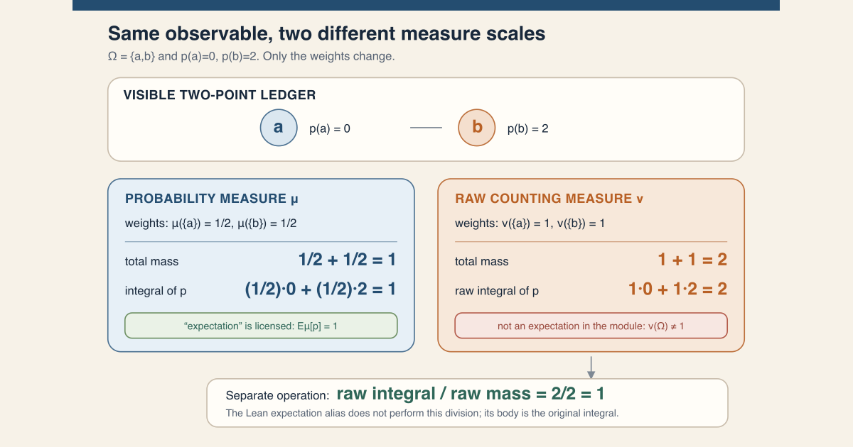
\[ \Omega=\{a,b\},\qquad p(a)=0,\qquad p(b)=2. \]Think of \(p\) as a tiny stand-in for a nonnegative finite-horizon observable. There are no hidden samples or limiting arguments. We will integrate the same two values against two different measures:
| point | observable \(p\) | probability weight \(\mu\) | raw weight \(\nu\) |
|---|---|---|---|
| \(a\) | \(0\) | \(1/2\) | \(1\) |
| \(b\) | \(2\) | \(1/2\) | \(1\) |
| total | not applicable | \(1\) | \(2\) |
For the probability measure,
\[ \int_\Omega p\,d\mu =\frac12\cdot0+\frac12\cdot2 =1. \]For the raw counting measure,
\[ \int_\Omega p\,d\nu =1\cdot0+1\cdot2 =2. \]The observable did not change. The scale of the measure did. Only the first integral is an expectation under the displayed measure because only \(\mu(\Omega)=1\).
This immediately separates two formulas that are often blurred:
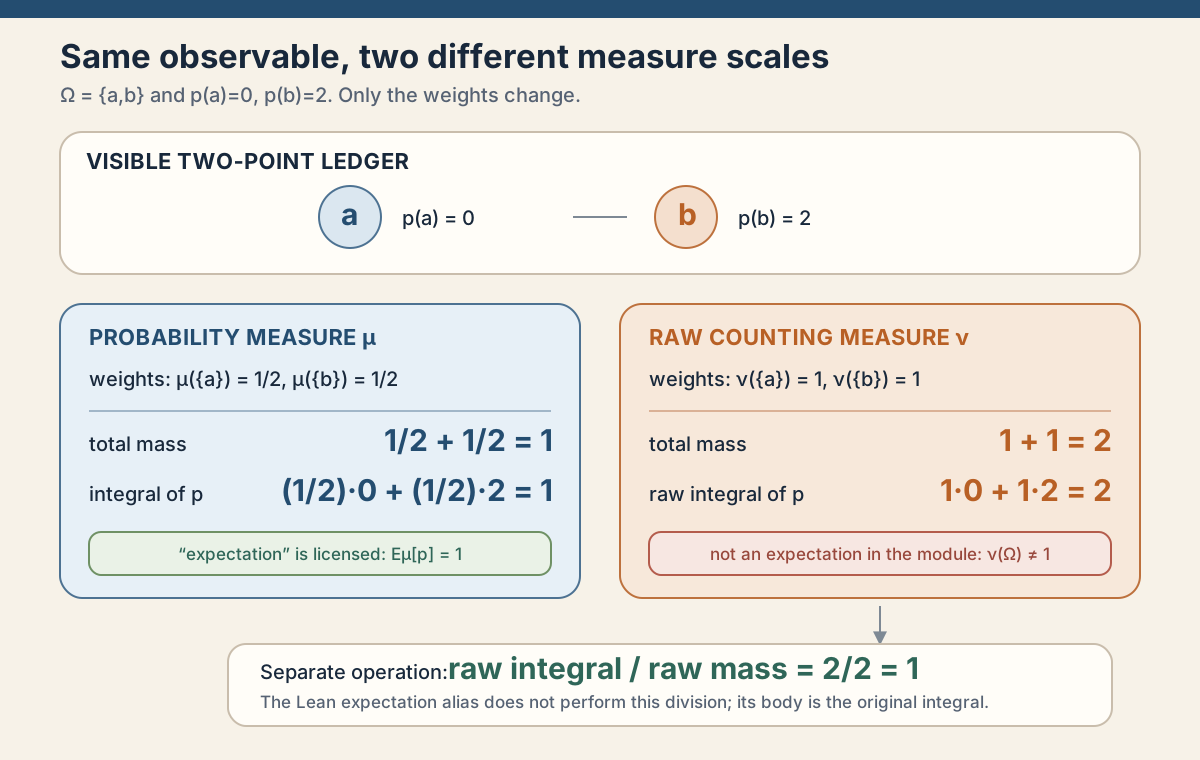
\[ \underbrace{\int p\,d\nu}_{\text{raw integral }=2} \qquad\text{and}\qquad \underbrace{\frac{\int p\,d\nu}{\nu(\Omega)}}_{\text{renormalized average }=1}. \]The project definition
finiteHorizonLogPlusExpectation performs the first operation.
Its [IsProbabilityMeasure μ] premise guarantees in advance that
the two operations coincide because \(\mu(\Omega)=1\).
Base camp continued: invariant information
Now keep the same two points and compare three dynamical systems:
- uniform probability \(\mu\) with the swap \(T(a)=b,\ T(b)=a\);
- the same probability with the identity map; and
- raw mass \(\nu\) with the swap.
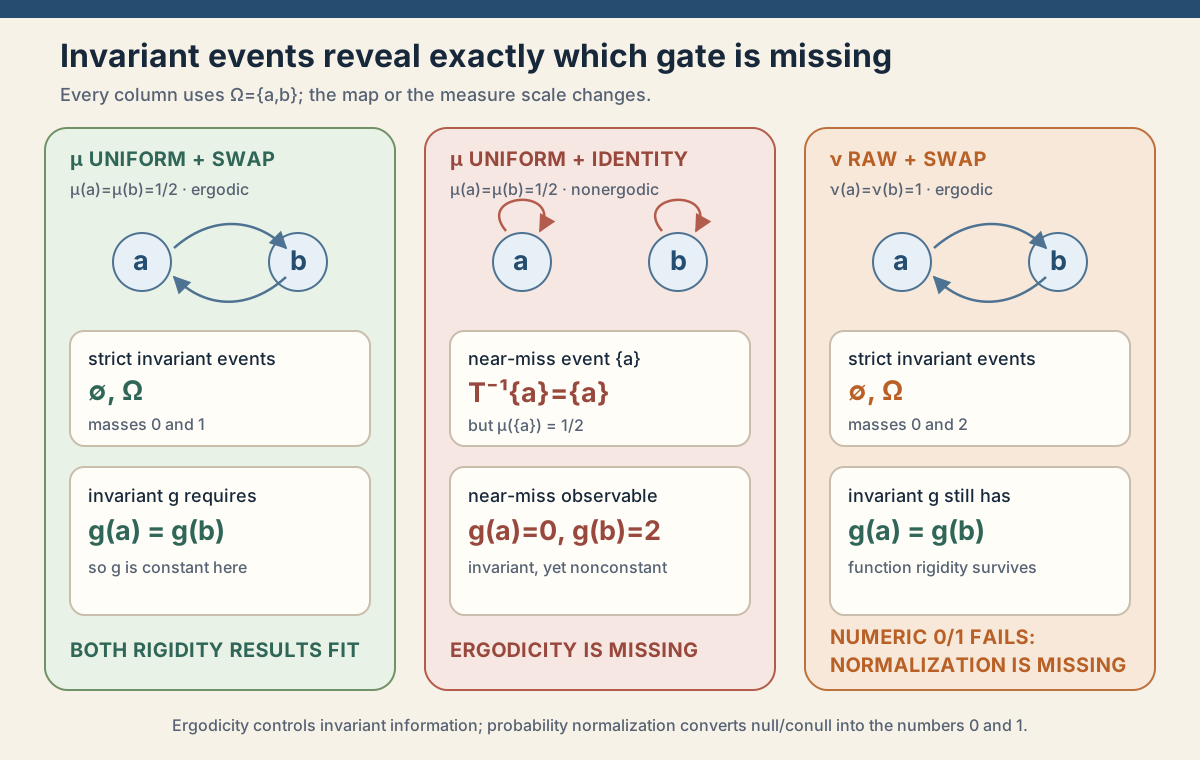
An event \(A\subseteq\Omega\) is strictly invariant when \(T^{-1}(A)=A\). In the swap system, the singletons trade places, so only \(\varnothing\) and \(\Omega\) are invariant. In the identity system, every event is invariant.
The complete finite ledger is:
| measure and map | strict invariant events | their masses | invariant \(g(a)=0,g(b)=2\)? |
|---|---|---|---|
| uniform \(\mu\), swap | \(\varnothing,\Omega\) | \(0,1\) | no |
| uniform \(\mu\), identity | all four events | \(0,\frac12,\frac12,1\) | yes, but nonconstant |
| raw \(\nu\), swap | \(\varnothing,\Omega\) | \(0,2\) | no |
On a finite space with positive weight at every point, “almost everywhere” means “at every point.” In general measure spaces, null sets may be nonempty, so the project theorem correctly concludes only almost-everywhere constancy. See null set , almost everywhere , and ergodic probability base before climbing into that distinction.
A boundary example: settled averages, oscillating outcomes
There is one more trap to remove at base camp. Define
\[ Y_n(a)=(-1)^n,\qquad Y_n(b)=-(-1)^n. \]Under the uniform probability measure,
\[ \int_\Omega Y_n\,d\mu=0 \]for every \(n\), so the integrated sequence is already constant. Yet \(Y_n(a)\) alternates \(1,-1,1,-1,\ldots\), and \(Y_n(b)\) alternates in the opposite phase. Neither sample path converges.
| horizon \(n\) | \(Y_n(a)\) | \(Y_n(b)\) | uniform mean |
|---|---|---|---|
| \(0\) | \(1\) | \(-1\) | \(0\) |
| \(1\) | \(-1\) | \(1\) | \(0\) |
| \(2\) | \(1\) | \(-1\) | \(0\) |
| \(3\) | \(-1\) | \(1\) | \(0\) |
This is deliberately not claimed to be a subadditive cocycle process. It is a counterexample only to the invalid inference
\[ \text{convergence of integrated scalars} \Longrightarrow \text{samplewise convergence}. \]Kingman’s theorem supplies far more structure than convergence of those scalars. RMT-17 does not supply that theorem.
From the ledger to the cocycle module
The sixteenth random-matrix-theory milestone (RMT-16) ended with a deterministic theorem. For the finite-horizon log-positive envelope
\[ P_k(\omega) {} = \log^+\lVert C(k,\omega)\rVert_\infty, \]it integrated first,
\[ I_k=\int_\Omega P_k(\omega)\,d\mu(\omega), \]proved the real sequence \(I_k\) subadditive, and obtained the positive-time Fekete rate
\[ \gamma_\mu^+(C) {} = \inf_{k\ge1}\frac{I_k}{k}. \]That proof removed the outcome variable before taking a limit. The next milestone, RMT-17, now prepares the probabilistic and ergodic vocabulary needed for later sample-dependent theorems, but it does not cross that later theorem boundary.
RMT-17 prepares three independent axes:
IsProbabilityMeasure μfixes total mass at one;Ergodic C.base μmakes invariant information trivial modulo null sets; andC.HasIntegrableGeneratorLogPluscontrols every finite-horizon positive-log moment.
The module exports one generic process-candidate structure, four deterministic rate facts, a probability-specialized expectation definition and equality, and two ergodic rigidity bridges. It exports no Kingman theorem, no samplewise limit, and no Lyapunov exponent.
Choose a route up
| Route | Begin with | Destination |
|---|---|---|
| First encounter | Two points expose the normalization | Recompute mass, integral, invariant events, and a nonergodic near miss |
| Probability route | Camp one: probability fixes scale | Learn exactly what mass one does and does not buy |
| Ergodic route | Camp two: ergodicity fixes invariant information | Read the event and function forms of rigidity |
| Analytic route | Camp three: integrability remains separate | Package the finite process without hidden asymptotics |
| Rate route | Camp four: four deterministic rate facts | Reuse Fekete without probability or ergodicity |
| Example route | Four models that separate the assumptions | Test every tempting implication on exact spaces |
| Cocycle route | The alternating scalar cocycle | Compute a nonmonotone normalized expectation and a strict rate bound |
| Hands-on Lean route | Type the two-point ledger | Run exact rational arithmetic and finite invariance checks with only Std |
| Lean route | The complete ten-declaration map | Audit every exported declaration in source order |
| Summit route | The pre-Kingman boundary | Identify the missing theorem and rule out automatic limit claims |
Learning objectives
By the summit, a reader should be able to:
- state
IsProbabilityMeasure μas the equation \(\mu(\Omega)=1\); - explain why probability normalization does not imply integrability, ergodicity, independence, or mixing;
- unpack
Ergodic T μinto measure preservation and invariant-set rigidity; - distinguish a null-or-conull event conclusion from the numerical probability zero-one conclusion;
- explain why the invariant-function theorem needs ergodicity but no probability typeclass;
- explain why
HasIntegrableGeneratorLogPlusis an independent analytic hypothesis; - read both fields of
IsIntegrableSubadditiveProcessCandidateexactly; - identify what that candidate deliberately does not store;
- derive nonnegativity of the deterministic integrated rate from convergence of nonnegative normalized values;
- read the positive-index infimum theorem without accidentally including time zero;
- derive the upper bound by every positive normalized horizon;
- specialize that bound to one step;
- explain why the expectation alias is definitionally the raw integral;
- identify the strict invariance and measurability requirements in the event zero-one theorem;
- identify the almost-everywhere invariance and strong measurability requirements in the function theorem;
- use exact one-point and two-point examples to refute false implications;
- compute the alternating scalar cocycle at horizons one, two, and three;
- explain why ergodicity does not imply mixing;
- separate a deterministic limit of integrated values from a samplewise limit;
- run the bounded two-point
Stdworksheet on a normal Mac or Linux host; and - list the obligations still needed before a formal Kingman application.
The assumption matrix
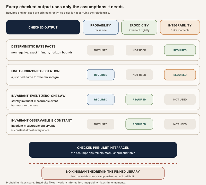
The matrix is more than editorial organization. It is a picture of the Lean signatures. If probability or ergodicity were silently used in the rate theorems, those theorems would have extra arguments. If probability were silently needed for invariant-function rigidity, that theorem would carry a typeclass premise. It does not.
Conversely, the expectation definition carries both probability and integrability even though its body is the same integral as before. Those arguments are not computational decorations. They encode the semantic and analytic conditions under which the word “expectation” is appropriate.
The common setup
Fix a measurable base space \(\Omega\), a measure \(\mu\), a finite matrix index type \(\iota\) with decidable equality, and a bundled one-sided discrete matrix cocycle \(C\). Its base map is
\[ T=C.\mathrm{base}:\Omega\to\Omega. \]The cocycle already stores that \(T\) is measurable and preserves \(\mu\), in the sense of Mathlib’s measure-preserving map interface. Its finite products satisfy the chronological split
\[ C(m+k,\omega) {} = C(k,T^m\omega)C(m,\omega). \]The selected matrix norm is the maximum absolute row-sum norm, and the positive logarithm is
\[ \log^+x=\max(\log x,0) \]with the project’s zero policy inherited from earlier modules. The resulting finite process is \(P:\mathbb N\to\Omega\to\mathbb R\).
Three propositions can now be asked without answering one another:
| Question | Lean witness | What it controls |
|---|---|---|
| Does the measure have unit mass? | [IsProbabilityMeasure μ] | Probability vocabulary and numerical zero-one values |
| Is invariant base information trivial? | hErg : Ergodic C.base μ | Invariant events and invariant observables |
| Are finite positive-log moments legitimate? | hC : C.HasIntegrableGeneratorLogPlus | Finite-horizon integrability and deterministic rate facts |
Measure preservation is a fourth fact, already bundled in \(C\). It makes shifted integrals agree and supports the previous scalar subadditivity proof. It does not imply any row of this table except its own statement.
In Lean: seven bridges from the ledger to the module
Each bridge pairs a human sentence, paper mathematics, exact Lean syntax, and the tokens a reader must recognize. The finite worksheet after the bridges checks the opening arithmetic. The project declarations themselves belong to the full project checks.
Bridge 1: say that the measure is normalized
[IsProbabilityMeasure μ]- Square brackets request automatic typeclass-instance synthesis.
IsProbabilityMeasureis the class whose defining field isμ univ = 1.μis still a general measure object; this premise fixes its scale.- The token says nothing by itself about integrability, independence, ergodicity, or mixing.
Bridge 2: expose the same integral as an expectation
finiteHorizonLogPlusExpectation_eq_integratedLogPlusNorm hC kfiniteHorizonLogPlusExpectationis the probability-facing name.integratedLogPlusNormis the earlier raw-integral name.hCsupplies finite-horizon integrability; it does not divide the integral by a mass.kis the finite horizon.- The theorem is proved by
rfl: both sides unfold to the same expression.
Bridge 3: read the analytic field of the candidate
hX.integrable khXis evidence forIsIntegrableSubadditiveProcessCandidate T μ X.- The dot selects its field named
integrable. kchooses one time slice \(X_k\).- The result is
Integrable (X k) μ, a genuine analytic premise, not a claim about totalized integral syntax.
Bridge 4: keep the base shift in subadditivity
hX.add_le m k ωadd_leis the candidate’s second and final stored field.mis the length of the first block andkthe next block.ωis one source outcome.- Lean writes the shift as
(T^[m]) ωin the elaborated theorem. - Removing that shift would describe an ordinary scalar subadditive sequence, not the intended dynamical process.
Bridge 5: identify the deterministic positive-time rate
hC.integratedLogPlusGrowthRate_eq_sInfhCis the one-step log-positive integrability witness.integratedLogPlusGrowthRatewas defined from Mathlib’s deterministic subadditive limit.sInfis the greatest lower bound of a set of real values.Ici 1is the set of natural horizons \(k\ge1\).- The theorem needs neither a probability instance nor an ergodicity proof.
Bridge 6: turn invariant-event rigidity into numbers zero or one
C.ergodicBase_invariantEvent_prob_eq_zero_or_one hErg hs hinvCsupplies the base mapC.base.hErgproves that base map ergodic for \(\mu\).hsproves the event is measurable.hinvhas the strict equalityC.base ⁻¹’ s = s.- The ambient
[IsProbabilityMeasure μ]converts conull mass into the number \(1\); the raw-swap example would instead give mass \(2\).
Bridge 7: make an invariant observable constant almost everywhere
C.ergodicBase_ae_eq_const_of_ae_invariant hErg hg hinvhgisAEStronglyMeasurable g μ.- Here
hinvis the almost-everywhere equalityg ∘ C.base =ᵐ[μ] g, not a set equality. =ᵐ[μ]means equality outside a \(\mu\)-null set.- The result produces a real constant
cand another almost-everywhere equality. - No probability typeclass appears: ergodic function rigidity is insensitive to multiplying the measure by a positive scalar.
Type the two-point ledger yourself with Lean and Std
The next file imports only Lean’s small Std library. It models
finite weighted sums with exact rational numbers, enumerates all four events,
checks invariance under the swap and identity maps, and prints the oscillating
mean ledger. It does not construct a Mathlib measure, matrix cocycle, or
Kingman theorem.
Save this exact text as
/tmp/ProbabilityErgodicBaseTutorial.lean:
import Std

namespace ProbabilityErgodicBaseTutorial

inductive Point where
  | a
  | b
  deriving Repr, DecidableEq

open Point

def points : List Point := [a, b]

def observable : Point → Rat
  | a => 0
  | b => 2

def probabilityWeight : Point → Rat
  | a => 1 / 2
  | b => 1 / 2

def rawWeight : Point → Rat
  | a => 1
  | b => 1

def finiteIntegral (weight : Point → Rat) (f : Point → Rat) : Rat :=
  (points.map fun ω => weight ω * f ω).sum

structure Event where
  hasA : Bool
  hasB : Bool
  deriving Repr, DecidableEq

def events : List Event :=
  [⟨false, false⟩, ⟨true, false⟩, ⟨false, true⟩, ⟨true, true⟩]

def Event.contains (s : Event) : Point → Bool
  | a => s.hasA
  | b => s.hasB

def identity : Point → Point := fun ω => ω

def swap : Point → Point
  | a => b
  | b => a

def invariantUnder (T : Point → Point) (s : Event) : Bool :=
  points.all fun ω => s.contains (T ω) == s.contains ω

def eventMass (weight : Point → Rat) (s : Event) : Rat :=
  (points.filter s.contains).map weight |>.sum

def invariantMasses (weight : Point → Rat) (T : Point → Point) : List Rat :=
  (events.filter (invariantUnder T)).map (eventMass weight)

def invariantObservableUnder (T : Point → Point) (f : Point → Rat) : Bool :=
  points.all fun ω => f (T ω) == f ω

def oscillatingValue (n : Nat) : Point → Int
  | a => if n % 2 = 0 then 1 else -1
  | b => if n % 2 = 0 then -1 else 1

def oscillatingMeanNumerator (n : Nat) : Int :=
  oscillatingValue n a + oscillatingValue n b

#eval finiteIntegral probabilityWeight (fun _ => 1)
#eval finiteIntegral probabilityWeight observable
#eval finiteIntegral rawWeight (fun _ => 1)
#eval finiteIntegral rawWeight observable
#eval invariantMasses probabilityWeight swap
#eval invariantMasses probabilityWeight identity
#eval invariantMasses rawWeight swap
#eval invariantObservableUnder swap observable
#eval invariantObservableUnder identity observable
#eval (List.range 6).map oscillatingMeanNumerator

example : finiteIntegral probabilityWeight (fun _ => 1) = 1 := by native_decide
example : finiteIntegral probabilityWeight observable = 1 := by native_decide
example : finiteIntegral rawWeight (fun _ => 1) = 2 := by native_decide
example : finiteIntegral rawWeight observable = 2 := by native_decide
example : invariantMasses probabilityWeight swap = [0, 1] := by native_decide
example : invariantMasses probabilityWeight identity = [0, 1 / 2, 1 / 2, 1] := by native_decide
example : invariantMasses rawWeight swap = [0, 2] := by native_decide
example : invariantObservableUnder swap observable = false := by native_decide
example : invariantObservableUnder identity observable = true := by native_decide
example : (List.range 6).map oscillatingMeanNumerator = [0, 0, 0, 0, 0, 0] := by native_decide

end ProbabilityErgodicBaseTutorial
Run it on an ordinary Mac or Linux host with the repository’s pinned Lean
version, without entering formalization/ and without invoking
Lake:
source "$HOME/.elan/env"
elan run leanprover/lean4:v4.32.0 lean \
  /tmp/ProbabilityErgodicBaseTutorial.lean
The exact file above was run successfully with Lean 4.32.0 and printed:
1
1
2
2
[0, 1]
[0, (1 : Rat)/2, (1 : Rat)/2, 1]
[0, 2]
false
true
[0, 0, 0, 0, 0, 0]
Read the lines in order: probability mass, probability integral, raw mass, raw integral, swap-invariant probability masses, identity-invariant probability masses, swap-invariant raw masses, whether the nonconstant observable survives the swap, whether it survives the identity, and the first six oscillating mean numerators.
Resource profile: small standalone tutorial, local-safe. The propositions
discharged by native_decide are kernel-checked instances of this
finite representation and its rational arithmetic. They do not prove the Mathlib-backed project
theorems. Those exact checks require the repository’s pinned Lean and Mathlib
dependencies.
Camp one: probability fixes scale
The exact Mathlib class
Mathlib defines a probability measure by one field:
class IsProbabilityMeasure (μ : Measure α) : Prop where
  measure_univ : μ univ = 1
The official probability-measure typeclass documentation also records consequences such as finiteness and nonzeroness. In particular, the typeclass prevents the total mass from being an arbitrary finite scalar.
This is a normalization condition on a measure. It is not a theorem about the base map \(T\). The identity map on a two-point uniform probability space is measure preserving but not ergodic. A periodic flip is ergodic but not mixing. Probability alone does not distinguish them.
It is also not a theorem about a measurable function’s tails. A real-valued function may be finite at every point of a probability space and still have a divergent absolute integral. The example \(x\mapsto1/x\) on \((0,1]\) will make that failure explicit below.
Why expectation needs two gates
RMT-16 defined the raw integral
\[ I_k=\int_\Omega P_k\,d\mu \]for an arbitrary measure. Mathlib’s Bochner integral is totalized, so this
expression has a real value even if \(P_k\) is not integrable. The separate
hC witness prevents that value from being misread as a finite
moment.
RMT-17 introduces
def finiteHorizonLogPlusExpectation [IsProbabilityMeasure μ]
    (C : DiscreteMatrixCocycle (ι := ι) μ)
    (_hC : C.HasIntegrableGeneratorLogPlus) (k : ℕ) : ℝ :=
  ∫ ω, C.logPlusNormObservable k ω ∂μ
The two extra premises do different jobs:
[IsProbabilityMeasure μ]makes the integral a probability expectation; and_hCsupplies genuine finite-horizon integrability through the RMT-15 propagation theorem.
The underscore in _hC means the proof term does not occur in the
definition’s computational body. It does not mean the assumption is
mathematically disposable. Its presence at the public boundary blocks callers
from applying expectation language to the totalized nonintegrable branch.
Declaration 8: the expectation is the raw integral
The next theorem is
@[simp] theorem finiteHorizonLogPlusExpectation_eq_integratedLogPlusNorm
    [IsProbabilityMeasure μ]
    {C : DiscreteMatrixCocycle (ι := ι) μ}
    (hC : C.HasIntegrableGeneratorLogPlus) (k : ℕ) :
    C.finiteHorizonLogPlusExpectation hC k = C.integratedLogPlusNorm k := by
  rfl
The proof is reflexivity because both sides unfold to the same integral. Probability normalization does not divide by total mass here. Total mass is already one. The theorem is a semantic bridge between two names for one scalar, not a numerical conversion formula.
This distinction matters when comparing raw measures. If the one-point base has mass two, \(I_k\) remains defined and may be finite, but RMT-17 does not offer the expectation name. Renormalizing that measure to mass one would be a separate construction with correspondingly rescaled integrals.
Camp two: ergodicity fixes invariant information
The event definition
Mathlib separates PreErgodic T μ from
Ergodic T μ. Pre-ergodicity says that every measurable set \(A\)
with strict preimage invariance
is almost everywhere empty or almost everywhere universal. Ergodicity extends that property with measure preservation. The official ergodic maps and measures documentation is the upstream authority for both structures.
The most primitive numerical statement is therefore not automatically “probability zero or one.” Before normalization, the invariant set satisfies
\[ \mu(A)=0 \quad\text{or}\quad \mu(A^c)=0. \]The second branch says \(A\) is conull. Its numerical mass equals the mass of the entire space, which may be two, seven, or infinite. Only on a probability space does the second branch become \(\mu(A)=1\).
Declaration 9: invariant-event probability is zero or one
RMT-17 exposes exactly that normalized bridge:
theorem ergodicBase_invariantEvent_prob_eq_zero_or_one
    [IsProbabilityMeasure μ]
    (C : DiscreteMatrixCocycle (ι := ι) μ)
    (hErg : Ergodic C.base μ) {s : Set Ω}
    (hs : MeasurableSet s) (hinv : C.base ⁻¹' s = s) :
    μ s = 0 ∨ μ s = 1
Every premise is visible:
- the measure has mass one;
- the base is ergodic;
- the event is measurable; and
- invariance is an exact set equality.
The theorem does not accept an arbitrary event whose probability happens to be preserved under one step. It requires the preimage set itself to be the same set. It also does not infer measurability from invariance.
The wrapper intentionally chooses a strict-invariance theorem even though Mathlib contains more general almost-invariant machinery through quasi-ergodicity. A narrow exact signature is easier to teach and audit at this stage. Future interfaces may relax the premise; the current theorem does not.
The function form of rigidity
An invariant event is a binary observable. The same idea extends to real-valued information. If a measurable \(g:\Omega\to\mathbb R\) satisfies \(g\circ T=g\), then each measurable threshold event associated with \(g\) is invariant. Ergodicity forces those threshold events to be trivial, which in turn forces \(g\) to be essentially constant.
Mathlib proves this through a general countable-separation argument for measurable target spaces and specializes it to almost-everywhere strongly measurable functions into metrizable spaces. The official invariant-function documentation gives the precise theorem used here.
Declaration 10: an invariant real observable is almost everywhere constant
RMT-17’s wrapper is
theorem ergodicBase_ae_eq_const_of_ae_invariant
    (C : DiscreteMatrixCocycle (ι := ι) μ)
    (hErg : Ergodic C.base μ) {g : Ω → ℝ}
    (hg : AEStronglyMeasurable g μ)
    (hinv : g ∘ C.base =ᵐ[μ] g) :
    ∃ c : ℝ, g =ᵐ[μ] Function.const Ω c
There is no probability premise. Ergodicity is fundamentally a null-or-conull statement, so essential constancy makes sense for a raw measure. On the one-point mass-two space, for example, every real observable is genuinely constant even though the measure is not probabilistic.
There is also no integrability premise. Almost-everywhere strong measurability is enough for this rigidity theorem. The resulting constant is not asserted to be the expectation of \(g\), because \(g\) need not be integrable and the measure need not have mass one.
The conclusion is existential and almost everywhere. It does not choose a canonical constant, prove uniqueness on a zero measure, or upgrade equality at every point. These omissions are correct. Almost-everywhere statements ignore null sets, and on the zero measure every two functions are almost everywhere equal.
Why these two wrappers are matrix-dimension free
The two ergodic bridges mention a matrix cocycle only to obtain its base map.
Their proofs never inspect a matrix entry, enumerate an index type, or use
decidable matrix equality. The Lean source explicitly omits the ambient
Fintype ι and DecidableEq ι instances around these
theorems.
That is proof engineering with mathematical meaning: invariant base information does not depend on matrix dimension. A later refactor could place these statements on a more generic measure-preserving dynamical-system interface without changing their content.
Camp three: integrability remains separate
The inherited one-step hypothesis
The proposition
C.HasIntegrableGeneratorLogPlus
means that the one-step positive-log envelope \(P_1\) is integrable. Earlier modules use the cocycle inequality and a finite orbit-sum majorant to prove that every \(P_k\) is integrable. Nothing about that propagation requires mass one or ergodicity.
This is exactly the right separation. Integrability is a tail condition on an observable with respect to a measure. Probability is only the normalization of that measure. Ergodicity is only the rigidity of invariant information under its preserved dynamics. Neither can control the size of an arbitrary measurable generator.
Declaration 1: the generic process candidate
RMT-17 begins with a generic predicate:
structure IsIntegrableSubadditiveProcessCandidate
    {Ω : Type uΩ} [MeasurableSpace Ω] (T : Ω → Ω) (μ : Measure Ω)
    (X : ℕ → Ω → ℝ) : Prop where
  integrable : ∀ k, Integrable (X k) μ
  add_le : ∀ m k ω, X (m + k) ω ≤ X k (T^[m] ω) + X m ω
The first field certifies an ordinary real-valued integral at every fixed natural horizon. The second field preserves the time shift created by splitting a one-sided cocycle product. In mathematical notation,
\[ X_{m+k}(\omega) \le X_k(T^m\omega)+X_m(\omega). \]The later block is evaluated at the shifted base point. Erasing that shift would change the process being described.
The structure is a proposition. It packages evidence and contributes no new runtime data. Its name ends in Candidate because it records a finite-time shape, not a completed ergodic theorem.
What the candidate omits
The generic package deliberately does not store:
- measurability or measure preservation of \(T\);
- probability normalization of \(\mu\);
- ergodicity of \(T\);
- independence or identical distribution;
- nonnegativity of \(X_k\);
- a two-parameter stationary process law;
- a pointwise or almost-everywhere limit;
- an integrable-norm (\(L^1\)) convergence conclusion;
- equality between an integrated rate and an integral of a limit; or
- any Lyapunov or invariant-splitting structure.
For the actual cocycle, measurability and preservation already live in \(C\), and log-positive nonnegativity lives in the preceding observable layer. A future Kingman theorem should take the additional assumptions it truly needs rather than forcing this small reusable predicate to guess them.
Declaration 2: the cocycle supplies the candidate
The constructor theorem is
theorem HasIntegrableGeneratorLogPlus.isIntegrableSubadditiveProcessCandidate
    {C : DiscreteMatrixCocycle (ι := ι) μ}
    (hC : C.HasIntegrableGeneratorLogPlus) :
    IsIntegrableSubadditiveProcessCandidate C.base μ
      C.logPlusNormObservable
Its two fields come directly from checked predecessor theorems:
hC.integrable_logPlusNormObservablesupplies integrability at every horizon; andC.logPlusNormObservable_add_lesupplies the shifted pointwise inequality.
The proof does not introduce probability or ergodicity. It packages facts already established for \(P_k\).
Camp four: four deterministic rate facts
The next four theorems sharpen the deterministic Fekete rate from RMT-16.
Every one requires hC. None requires probability or ergodicity.
The official
Mathlib subadditive-sequence interface supplies the
underlying positive-index infimum and comparison theorem.
Declaration 3: the rate is nonnegative
Every normalized integrated value satisfies
\[ A_k=\frac{I_k}{k}\ge0. \]RMT-16 proved \(A_k\to\gamma_\mu^+(C)\). RMT-17 passes nonnegativity through that limit:
\[ 0\le\gamma_\mu^+(C). \]The Lean proof uses ge_of_tendsto with the eventually true fact
that every term is nonnegative. This is a topological limit argument, not a
probability argument.
Positive clipping determines the sign and scope of the conclusion. A contraction-sensitive logarithmic rate can be negative, but \(P_k=\log^+\lVert C(k,\omega)\rVert\) cannot. The theorem therefore concerns only the clipped integrated rate.
Declaration 4: expose the exact positive-time infimum
RMT-17 unfolds the inherited definition as
\[ \gamma_\mu^+(C) {} = \inf\left\{A_k:k\ge1\right\}. \]The exact Lean right-hand side is
sInf (C.normalizedIntegratedLogPlusNorm '' Ici 1)
Here Ici 1 is the set of natural horizons at least one, and the
image maps those horizons through the normalized sequence. Time zero is not
part of this set.
This theorem matters because \(A_0=0\) by totalized division. If the infimum were taken over the full range, every nonnegative example would have infimum zero even when every positive-time ratio were strictly positive. The positive-index restriction carries real mathematical content.
Declaration 5: every positive horizon is an upper bound
For every natural \(k\ne0\),
\[ \gamma_\mu^+(C)\le A_k. \]This follows from the Fekete infimum, but the Lean proof uses Mathlib’s
Subadditive.lim_le_div theorem together with the lower bound on
the normalized range. The explicit premise \(k\ne0\) prevents accidental
division-by-zero interpretation.
The theorem does not say the ratios decrease. It says the limiting infimum is below each positive ratio. A sequence can move down, then up, and still obey that comparison. The alternating scalar example below has exactly this shape.
Declaration 6: the one-step moment is an upper bound
Specializing declaration 5 to \(k=1\) gives
\[ \gamma_\mu^+(C) \le A_1 {} = I_1. \]The equality uses division by one. On a probability base, \(I_1\) may be
called \(\mathbb E[P_1]\), provided hC is present. On an arbitrary
raw measure it remains an integrated value.
The upper bound can be strict. Later products can cancel one-step expansion, and positive clipping can erase the contracting half of an alternating cycle. The two-point flip will produce \(\gamma_\mu^+(C)=0\) while \(I_1=\log2/2\).
What these rate facts still do not use
| Assumption | Used by declarations 3 through 6? | Reason |
|---|---|---|
| One-step log-positive integrability | Yes | It underwrites scalar subadditivity and the inherited Fekete rate |
| Measure preservation | Already inside the cocycle | It was used upstream to remove shifts inside integrals |
| Probability normalization | No | Fekete acts on a real sequence for any raw measure |
| Ergodicity | No | The outcome variable was integrated away before the limit |
| Independence | No | Subadditivity and preserved integrals suffice |
| Mixing | No | No correlation limit enters the proof |
This ledger prevents a common historical overread. A theorem may sit in a random-cocycle namespace and be motivated by random products while remaining entirely deterministic after integration.
Four models that separate the assumptions
Small exact models are the quickest defense against false implication arrows. The first three examples use finite spaces, where every set is measurable, every finite-valued function is integrable against a finite measure, and the invariant subsets can be listed by hand. The fourth uses a continuum to show that probability normalization does not control integrable tails.
Model A: probability without ergodicity
Let
\[ \Omega=\{0,1\}, \qquad \mu(\{0\})=\mu(\{1\})=\frac12, \qquad T=\operatorname{id}. \]The measure has total mass one, and the identity preserves it. Every subset is strictly invariant. In particular, \(A=\{0\}\) satisfies
\[ T^{-1}(A)=A, \qquad \mu(A)=\frac12. \]If the base were ergodic, declaration 9 would force this mass to be zero or one. It is neither. Thus probability and measure preservation do not imply ergodicity.
An invariant real observable makes the same failure visible. Define \(g(0)=0\) and \(g(1)=1\). Since \(T\) is the identity, \(g\circ T=g\), but \(g\) is not almost everywhere constant. The missing premise is ergodicity, not measurability or integrability.
Model B: ergodicity without probability
Let
\[ \Omega=\{\ast\}, \qquad \mu(\{\ast\})=2, \qquad T=\operatorname{id}. \]The identity preserves every measure. The only subsets are empty and full, so every measurable invariant set is null or conull. The base is ergodic.
It is not a probability base because \(\mu(\Omega)=2\). Declaration 10 still applies: every real observable is constant. Declaration 9 does not apply, and should not. Its full invariant event has mass two, so the numerical conclusion “zero or one” would be false.
This model explains why Ergodic T μ cannot secretly include
IsProbabilityMeasure μ in Mathlib’s design.
Model C: probability and ergodicity without mixing
Use the uniform two-point probability measure again and define the flip
\[ T(0)=1, \qquad T(1)=0. \]The flip preserves the measure. A strictly invariant subset must contain both points or neither, so the base is ergodic.
Now take \(A=\{0\}\). Its pullbacks alternate:
\[ T^{-n}(A) {} = \begin{cases} A,& n\text{ even},\\ \{1\},& n\text{ odd}. \end{cases} \]Consequently,
\[ \mu\bigl(A\cap T^{-n}(A)\bigr) {} = \begin{cases} \tfrac12,& n\text{ even},\\ 0,& n\text{ odd}. \end{cases} \]Mixing would require this quantity to converge to \(\mu(A)\mu(A)=1/4\). It alternates forever. The system is ergodic and not mixing.
This is not a contradiction. Ergodicity controls time-invariant information. Mixing controls asymptotic decorrelation, which is stronger and absent from RMT-17.
Model D: probability without integrability
Let \(\Omega=(0,1]\) with Lebesgue probability measure and let the base map be the identity. Define a one-dimensional measurable generator by
\[ G(x)=\begin{bmatrix}\exp(1/x)\end{bmatrix}. \]Every matrix entry is finite at every base point. The one-step positive-log envelope is
\[ P_1(x)=\frac1x. \]But
\[ \int_0^1\frac{dx}{x}=+\infty. \]Thus the probability typeclass can hold while
HasIntegrableGeneratorLogPlus fails. The base is also not
ergodic because the identity leaves every measurable set invariant, but that
is not responsible for the divergent moment.
Conversely, put any finite-valued generator on the mass-two, two-point identity space. The one-step envelope is integrable automatically, while the measure is not probabilistic and the identity is not ergodic. Integrability does not force either dynamical property.
The alternating scalar cocycle
The most informative calibration combines Model C’s ergodic flip with a one-dimensional cocycle. Set
\[ G(0)=\begin{bmatrix}2\end{bmatrix}, \qquad G(1)=\begin{bmatrix}\tfrac12\end{bmatrix}. \]Because the base alternates, adjacent generators cancel. Starting at zero, the products are
\[ C(1,0)=\begin{bmatrix}2\end{bmatrix}, \qquad C(2,0)=\begin{bmatrix}1\end{bmatrix}, \qquad C(3,0)=\begin{bmatrix}2\end{bmatrix}. \]Starting at one, they are
\[ C(1,1)=\begin{bmatrix}\tfrac12\end{bmatrix}, \qquad C(2,1)=\begin{bmatrix}1\end{bmatrix}, \qquad C(3,1)=\begin{bmatrix}\tfrac12\end{bmatrix}. \]Every even-horizon product is one from either starting point. At odd horizons, the product is two from zero and one half from one. Positive logarithmic clipping therefore gives
\[ P_{2r}(0)=P_{2r}(1)=0, \]and
\[ P_{2r+1}(0)=\log2, \qquad P_{2r+1}(1)=0. \]All functions are integrable because the probability space is finite. Let
\[ E_k=\mathbb E_\mu[P_k], \qquad Q_k=\frac{E_k}{k} \quad(k\ge1). \]Then
\[ E_{2r}=0, \qquad E_{2r+1}=\frac{\log2}{2}, \]so the first three normalized values are
\[ Q_1=\frac{\log2}{2}, \qquad Q_2=0, \qquad Q_3=\frac{\log2}{6}. \]The sequence drops and then rises. Fekete convergence does not require monotone normalized ratios.
Every even positive horizon contributes zero to the positive-index infimum, while all normalized values are nonnegative. Hence
\[ \gamma_\mu^+(C)=0. \]The one-step upper bound is strict:
\[ \gamma_\mu^+(C) {} = 0 \lt \frac{\log2}{2} {} = E_1. \]This one model has probability normalization, ergodicity, finite-horizon integrability, and the subadditive-process candidate. It illustrates every new rate comparison and expectation bridge. Yet the RMT-17 Lean module proves no convergence of \(P_k(\omega)/k\) for this model or for general cocycles. One may perform additional arithmetic outside the module, but that cannot be misreported as a theorem exported by RMT-17.
The model is also not mixing, as Model C showed. Thus even the full RMT-17 assumption palette does not silently contain decay of correlations.
The complete ten-declaration map
The public interface has ten source-level declarations when the process structure is counted once. Its two field projections are generated from that structure and are taught under declaration 1.
| No. | Lean declaration | Explicit assumptions | Exact conclusion |
|---|---|---|---|
| 1 | IsIntegrableSubadditiveProcessCandidate | A measurable base type, map, measure, and real process | Stores all-horizon integrability and the shifted subadditive inequality |
| 2 | HasIntegrableGeneratorLogPlus.isIntegrableSubadditiveProcessCandidate | hC | Packages the cocycle’s log-positive process as the candidate |
| 3 | HasIntegrableGeneratorLogPlus.integratedLogPlusGrowthRate_nonneg | hC | \(0\le\gamma_\mu^+(C)\) |
| 4 | HasIntegrableGeneratorLogPlus.integratedLogPlusGrowthRate_eq_sInf | hC | The rate is the infimum of normalized values over \(k\ge1\) |
| 5 | HasIntegrableGeneratorLogPlus.integratedLogPlusGrowthRate_le_normalized | hC and \(k\ne0\) | The rate is at most the \(k\)-horizon normalized integral |
| 6 | HasIntegrableGeneratorLogPlus.integratedLogPlusGrowthRate_le_oneStep | hC | The rate is at most the one-step integrated envelope |
| 7 | finiteHorizonLogPlusExpectation | Probability and hC | Names the finite-horizon integral as an expectation |
| 8 | finiteHorizonLogPlusExpectation_eq_integratedLogPlusNorm | Probability and hC | Proves the expectation name and raw integral are definitionally equal |
| 9 | ergodicBase_invariantEvent_prob_eq_zero_or_one | Probability, ergodicity, event measurability, and strict invariance | The event has probability zero or one |
| 10 | ergodicBase_ae_eq_const_of_ae_invariant | Ergodicity, almost-everywhere strong measurability, and almost-everywhere invariance | The real observable is almost everywhere constant |
The table has no row labeled “samplewise convergence.” That is not an omitted documentation detail. It is an absent theorem.
Assumption ledger by theorem family
| Property | Process candidate | Rate facts | Expectation bridge | Event bridge | Function bridge |
|---|---|---|---|---|---|
| Measurable base space | Yes | Yes, through the cocycle | Yes | Yes | Yes |
| Base measure preservation | Not stored generically | Already in the cocycle | Already in the cocycle | Included in ergodicity and the cocycle | Included in ergodicity and the cocycle |
| Probability normalization | No | No | Yes | Yes | No |
| Base ergodicity | No | No | No | Yes | Yes |
| One-step log-positive integrability | Used for the cocycle constructor | Yes | Yes | No | No |
| Event measurability | Not applicable | Not applicable | Not applicable | Yes | Not applicable |
| Exact event invariance | Not applicable | Not applicable | Not applicable | Yes | Not applicable |
| Almost-everywhere strong measurability | Implied for each integrable process slice | Not a separate premise | Inherited from integrability | Not applicable | Yes |
| Almost-everywhere function invariance | Not applicable | Not applicable | Not applicable | Not applicable | Yes |
| Independence | No | No | No | No | No |
| Mixing | No | No | No | No | No |
“Not stored generically” is different from “false.” The generic candidate can be paired later with a map that is measurable and measure preserving. RMT-17 keeps that dynamical evidence in its natural owner rather than duplicating it inside the process predicate.
The pre-Kingman boundary
What Kingman’s theorem changes
Kingman’s subadditive ergodic theorem studies subadditive stochastic processes and supplies sample-dependent asymptotic conclusions under additional hypotheses (Kingman, 1968). In a one-parameter dynamical formulation, the characteristic finite-time inequality resembles
\[ X_{m+k}(\omega) \le X_k(T^m\omega)+X_m(\omega). \]That resemblance motivates the RMT-17 candidate. It is not itself a proof of the theorem. A formal application still needs an exact Lean theorem with an exact hypothesis list, codomain, measurability convention, and conclusion.
The distinction between deterministic Fekete and Kingman is an order-of-operations distinction:
\[ \text{RMT-16 and RMT-17:} \quad P_k(\omega) \longrightarrow \int P_k\,d\mu \longrightarrow \lim_k\frac1k\int P_k\,d\mu, \]whereas a samplewise theorem would study
\[ \text{later project route, completed at RMT-32:} \quad P_k(\omega) \longrightarrow \lim_k\frac{P_k(\omega)}{k} \quad\text{for almost every }\omega. \]The first limit is a limit of real numbers. The second is a limit of outcome-dependent values. Neither statement logically substitutes for the other.
What the pinned library supplies
The pinned Mathlib revision supplies:
- probability-measure typeclasses;
- measure-preserving, pre-ergodic, and ergodic structures;
- zero-one results for invariant events;
- almost-everywhere constancy for invariant functions; and
- deterministic subadditive-sequence Fekete machinery.
The local source audit found no Kingman or subadditive ergodic theorem matching this process. RMT-17 therefore exposes the native pieces that exist and stops. It does not add an axiom, cite a paper as if it were Lean code, or use an unverified theorem name.
Obligations the later formal theorem had to settle
From the viewpoint of RMT-17, crossing the bridge required the project to settle at least these choices:
- Process convention. Decide whether the theorem consumes a one-parameter family \(X_k\) with a base shift or a two-parameter process \(X_{m,n}\).
- Measure assumptions. State probability or finite-measure normalization exactly rather than hiding it behind expectation notation.
- Transformation assumptions. Supply measurability and measure preservation, and decide whether ergodicity is required for existence or only for constancy of the limit.
- Integrability assumptions. Match the theorem’s positive- and negative-part hypotheses. The actual \(P_k\) is nonnegative and integrable, but the generic candidate does not store nonnegativity.
- Measurability convention. Decide whether ordinary, almost-everywhere, or strong measurability is the theorem’s interface.
- Limit codomain. Decide whether the limit is real or extended real and how infinite values are ruled out.
- Invariant limit. Prove the limiting observable is invariant in the sense required by the ergodic constancy bridge.
- Integrated identification. Do not equate the integral of a limit with the limit of integrals without the exact convergence or uniform integrability result that licenses it.
- Cocycle interpretation. Keep positive clipping explicit. Even a samplewise limit of \(P_k/k\) would still not recover negative contraction.
- Library integration. Prove the theorem in Lean against the pinned interfaces before any Knowledge Base page reports it as formalized.
This list is not bureaucratic overhead. Each item blocks a familiar but invalid
shortcut. Later milestones RMT-18 through RMT-32 now address this route in
separate modules, culminating in a project-local log-positive Kingman
endpoint. That later success does not retroactively put a samplewise theorem
inside ProbabilityErgodicBase.lean, and it does not turn the
deterministic Fekete theorem into that endpoint.
Why ergodic constancy cannot manufacture the limit
Declaration 10 has the logical form
\[ \text{measurable }g \quad+\quad g\circ T=g\text{ almost everywhere} \quad\Longrightarrow\quad g\text{ is almost everywhere constant}. \]It begins with a function \(g\). A future samplewise limit would first need to be constructed, proved measurable, and proved invariant. Ergodicity can then remove its residual dependence on \(\omega\). It cannot conjure \(g\) from a sequence whose convergence has not been proved.
The same order appears in classical ergodic theory: existence, invariance, and ergodic constancy are distinct proof stages. RMT-17 formalizes the last-stage rigidity interface, not the first-stage existence theorem.
Why the deterministic rate cannot identify a samplewise exponent
The deterministic rate is
\[ \gamma_\mu^+(C) {} = \lim_{k\to\infty}\frac1k\int P_k\,d\mu. \]Suppose a separate theorem produces an almost-everywhere limit \(L(\omega)=\lim_k P_k(\omega)/k\). The equality
\[ \int L\,d\mu=\gamma_\mu^+(C) \]would still need justification. Pointwise convergence alone does not permit interchanging limit and integral. A suitable theorem may package the needed integral conclusion, or a later proof may establish stronger convergence. RMT-17 does neither.
Random-matrix-product history makes this destination important. Furstenberg and Kesten study asymptotic products under probabilistic hypotheses (Furstenberg and Kesten, 1960), while Oseledets develops characteristic exponents and invariant splittings (Oseledets, 1968). Those results motivate the roadmap but cannot be inherited from a finite-time candidate by vocabulary.
Common wrong turns
Treating probability as randomness plus independence
IsProbabilityMeasure μ says only that total mass is one. The
two-point identity and two-point flip share the same probability measure and
have very different dynamics. No independence relation appears in the class.
Treating measure preservation as ergodicity
The identity preserves every measure. On a nontrivial probability space it leaves every event invariant, so it is typically the opposite of ergodic.
Treating ergodicity as mixing
The two-point flip is ergodic and periodic. Its event correlations alternate instead of converging. Mixing is not a synonym for invariant-set rigidity.
Treating ergodicity as a moment bound
Ergodicity says which invariant events are trivial. It does not bound an
arbitrary generator near a singularity or in a heavy tail. Keep
hC explicit.
Calling every raw integral an expectation
An expectation is an integral against a probability measure. RMT-17 exposes
that name only under [IsProbabilityMeasure μ], and retains
hC so the finite moment is genuine.
Thinking the expectation equality performs normalization
The equality theorem is rfl. It does not divide by
\(\mu(\Omega)\). The measure is already normalized by the typeclass premise.
Reading the process candidate as a theorem-ready black box
The candidate stores two finite-time facts. It omits preservation, probability, ergodicity, nonnegativity, and every asymptotic conclusion. Its name says “candidate” for a reason.
Removing the base shift from subadditivity
The correct inequality contains \(X_k(T^m\omega)\). Preservation can remove the shift after integration, but no pointwise theorem identifies it with \(X_k(\omega)\).
Including time zero in the rate infimum
The normalized definition is total and has \(A_0=0\). The rate infimum uses only \(k\ge1\). Including zero can change a positive answer to zero.
Saying normalized ratios decrease
The alternating scalar cocycle has \(Q_1\gt Q_2\lt Q_3\). The rate remains below every positive ratio, but consecutive ratios need not be ordered.
Using event rigidity to prove function constancy without measurability
Threshold events must be measurable for the invariant-set argument to work. RMT-17 asks for almost-everywhere strong measurability of the real observable.
Turning almost-everywhere constancy into pointwise constancy
Null sets remain invisible. The theorem returns an almost-everywhere equality, not a universal equality.
Claiming Kingman from the shape of the inequality
A familiar hypothesis pattern is not a checked theorem application. The pinned library has no matching Kingman declaration, and RMT-17 states no samplewise conclusion.
Calling the clipped rate a Lyapunov exponent
Positive clipping maps contraction and exact collapse to zero. A full Lyapunov theory needs contraction-sensitive logarithms and stronger asymptotic structure.
Exercises from base camp to theorem design
Base camp
- State the fields of
IsProbabilityMeasure μandErgodic T μin words. - Explain why a conull event need not have mass one on a raw measure.
- List the four premises of the RMT-17 event zero-one theorem.
- List the three premises of the invariant-function theorem after the cocycle is fixed.
- Explain why no probability premise occurs in declaration 10.
- Explain why
_hCcan be computationally unused but mathematically necessary in declaration 7.
Mid-mountain
- Enumerate the invariant subsets of the two-point identity and flip.
- Use \(A=\{0\}\) to prove the two-point flip is not mixing.
- On the one-point mass-two space, evaluate the masses of the empty and full invariant events.
- Verify that \(1/x\) is finite pointwise but not integrable on \((0,1]\).
- Explain why the process candidate does not need to duplicate measure preservation already stored by the cocycle.
- Derive the one-step rate bound from the positive-horizon comparison.
- Explain why the infimum theorem excludes zero even though the lower-bound theorem may use the full normalized range.
- Give a second numerical subadditive sequence whose normalized ratios are not monotone.
Summit
- Compute every product in the alternating scalar cocycle through horizon four from both starting points.
- Derive the formulas for \(E_{2r}\), \(E_{2r+1}\), and the rate.
- Identify which RMT-17 theorem families survive if probability is removed.
- Identify which theorem families survive if ergodicity is removed.
- Design a future theorem signature that consumes the candidate, base preservation, and probability without assuming ergodicity. State what its limiting conclusion may still depend on.
- Add ergodicity to that hypothetical signature and explain which separate proof would make the limit constant.
- State a condition that could justify interchanging a samplewise limit and expectation, without claiming RMT-17 proves it.
- Explain why a limit of log-positive norms would still miss negative contraction rates.
- Compare the roles of Kingman, Furstenberg-Kesten, and Oseledets without collapsing their conclusions.
- Audit the ten-declaration table against the Lean source and identify every assumption that appears in a signature but not a computational body.
Full project checks
The local Std file checks the finite ledger only. The following
two checks inspect the actual Mathlib-backed project declarations. Install the
repository’s pinned dependencies first; these checks may require substantial
disk space and memory.
The ten declarations in this chapter
The authoritative source is
formalization/NonlinearDynamics/Random/RandomCocycles/ProbabilityErgodicBase.lean.
Put this probe in a temporary project scratch file:
import NonlinearDynamics.Random.RandomCocycles.ProbabilityErgodicBase

open MeasureTheory Set Filter
open NonlinearDynamics.Random.RandomCocycles
open NonlinearDynamics.Random.RandomCocycles.DiscreteMatrixCocycle

#print IsIntegrableSubadditiveProcessCandidate
#check HasIntegrableGeneratorLogPlus.isIntegrableSubadditiveProcessCandidate
#check HasIntegrableGeneratorLogPlus.integratedLogPlusGrowthRate_nonneg
#check HasIntegrableGeneratorLogPlus.integratedLogPlusGrowthRate_eq_sInf
#check HasIntegrableGeneratorLogPlus.integratedLogPlusGrowthRate_le_normalized
#check HasIntegrableGeneratorLogPlus.integratedLogPlusGrowthRate_le_oneStep
#check finiteHorizonLogPlusExpectation
#check finiteHorizonLogPlusExpectation_eq_integratedLogPlusNorm
#check ergodicBase_invariantEvent_prob_eq_zero_or_one
#check ergodicBase_ae_eq_const_of_ae_invariant
#print exposes both candidate fields. Each #check
elaborates one existing public declaration and shows its complete
type. The list contains the one structure plus the other nine source-level
declarations, in source order.
Full project check: exact repository module plus Mathlib. From the repository root, run:
cd formalization
lake env lean NonlinearDynamics/Random/RandomCocycles/ProbabilityErgodicBase.lean
This uses the repository’s pinned toolchain and dependencies to check the complete leaf.
cd formalization
lake env lean -DwarningAsError=true NonlinearDynamics/Random/RandomCocycles/ProbabilityErgodicBase.lean
Resource note: this exact file uses the repository's
pinned Lean and Mathlib dependencies. Initial project setup can require
substantial disk space and build time. For a lightweight first step on
macOS or Linux, use the page's standalone Lean-core or Std
tutorial.
The deterministic predecessor that supplies the rate
The immediate predecessor is
formalization/NonlinearDynamics/Random/RandomCocycles/IntegratedLogPlusGrowth.lean.
This smaller probe shows where the scalar sequence, normalization, rate, and
deterministic convergence theorem originate:
import NonlinearDynamics.Random.RandomCocycles.IntegratedLogPlusGrowth

open MeasureTheory Set Filter
open NonlinearDynamics.Random.RandomCocycles.DiscreteMatrixCocycle

#check integratedLogPlusNorm
#check HasIntegrableGeneratorLogPlus.integratedLogPlusNorm_add_le
#check HasIntegrableGeneratorLogPlus.subadditive_integratedLogPlusNorm
#check normalizedIntegratedLogPlusNorm
#check integratedLogPlusGrowthRate
#check HasIntegrableGeneratorLogPlus.tendsto_normalizedIntegratedLogPlusNorm
From the repository root, check this leaf with:
cd formalization
lake env lean NonlinearDynamics/Random/RandomCocycles/IntegratedLogPlusGrowth.lean
The last declaration proves convergence of the deterministic real sequence \(I_k/k\). It quantifies over no surviving outcome \(\omega\), so it cannot be relabelled as a samplewise theorem.
cd formalization
lake env lean -DwarningAsError=true NonlinearDynamics/Random/RandomCocycles/IntegratedLogPlusGrowth.lean
Resource note: this exact file uses the repository's
pinned Lean and Mathlib dependencies. Initial project setup can require
substantial disk space and build time. For a lightweight first step on
macOS or Linux, use the page's standalone Lean-core or Std
tutorial.
Automated success does not complete review of this public working note. Human mathematical, source, accessibility, and editorial reviews remain pending.
What is established and what is not
| Topic | RMT-17 status |
|---|---|
| Generic all-horizon integrable subadditive-process candidate | Defined |
| Cocycle log-positive process satisfies the candidate | Proved under hC |
| Deterministic integrated rate nonnegative | Proved under hC |
| Rate equals the positive-index infimum | Proved under hC |
| Rate below every positive normalized horizon | Proved under hC |
| Rate below the one-step integrated envelope | Proved under hC |
| Finite-horizon expectation name | Defined under probability and hC |
| Expectation equals the raw integrated value | Proved definitionally |
| Measurable strictly invariant event has probability zero or one | Proved under probability and ergodicity |
| Almost-everywhere invariant measurable real observable is almost everywhere constant | Proved under ergodicity |
| Probability implies ergodicity | False, refuted by the two-point identity |
| Ergodicity implies probability | False, refuted by the one-point mass-two base |
| Ergodicity implies mixing | False, refuted by the two-point flip |
| Probability implies integrability | False, refuted by the \(1/x\) envelope |
| Independence or identical distribution | Not assumed or proved |
| Mixing or correlation decay | Not assumed or proved |
| Samplewise normalized limit in RMT-17 | Not proved |
| Almost-everywhere, probability, distributional, or \(L^1\) convergence in RMT-17 | Not proved |
| Limit-expectation interchange | Not proved |
| Kingman theorem in the RMT-17 module | Not present in pinned Mathlib and not invoked; a later project-local endpoint appears at RMT-32 |
| Furstenberg-Kesten random-product theorem | Not invoked |
| Lyapunov exponent or Oseledets splitting | Not defined or proved |
The exact achievement is an assumption-safe interface. Probability fixes the scale of the measure. Ergodicity controls invariant information. Integrability controls finite moments. The deterministic Fekete facts remain deterministic, and the samplewise summit remains visibly ahead at this milestone. The current repository reaches that later summit only after fifteen additional formal layers.
Where to continue
The ergodic probability base entry is the compact definition, finite-example set, and caveat ledger for this chapter.
Ergodic Birkhoff Limits and Normalized Space Averages is the later additive endpoint. It uses pre-ergodicity to identify invariant conditional expectation and full ergodicity to obtain orbit convergence. That success does not fill this chapter’s separate Kingman and cocycle-growth gap.
Integrated Log-Positive Cocycle Growth and Its Deterministic Fekete Limit is the immediate predecessor. It constructs the raw integrated sequence and proves deterministic Fekete convergence.
Finite-Horizon Log-Positive Cocycle Integrability develops the one-step hypothesis and finite orbit majorant consumed by the process-candidate constructor.
Probability and Ergodic Base Interfaces for Matrix Cocycles is the proof-to-prose Research Note paired directly with the Lean module.
Finite Block Decomposition for Subadditive Processes is the immediate successor. It turns shifted subadditivity into two finite block-and-remainder Birkhoff bounds while keeping every asymptotic claim outside the theorem boundary.
Birkhoff Convergence Events Before the Pointwise Ergodic Theorem returns to this chapter’s rigidity interface after the intervening finite block, centering, phase, and packing milestones. It builds the exact invariant event where ordinary Birkhoff averages converge, then stops before selecting the conull branch.
The intervening asymptotic milestones supply pointwise and then subadditive convergence infrastructure. None permits a reader to rename the RMT-17 candidate itself as Kingman convergence.
Subadditive Upper Limsup Bounds Before Kingman Convergence now supplies one such later layer. It uses the probability and ergodic gates to prove the upper limsup half for a nonnegative process and preserves the missing lower-bound and convergence boundary.
The Guarded Real-Liminf Bridge to Log-Positive Kingman Convergence is the RMT-32 endpoint. It combines the later lower-liminf and upper-limsup layers to prove almost-everywhere convergence of the normalized log-positive cocycle observable. Read it only after this chapter: the endpoint depends on all three gates separated here, and it still proves neither a signed Lyapunov exponent nor an Oseledets splitting.
References
Mathlib contributors.
Probability-measure typeclasses,
Mathlib 4 documentation. This official source defines
IsProbabilityMeasure μ by \(\mu(\Omega)=1\), derives the
zero-or-probability and finite-measure instances, and records nonzeroness.
Mathlib contributors.
Ergodic maps and measures,
Mathlib 4 documentation. This official source defines PreErgodic
and Ergodic, gives null-or-conull invariant-set results, and proves
the probability zero-one specialization used by RMT-17.
Mathlib contributors. Functions invariant under an ergodic map, Mathlib 4 documentation. This official source proves that an almost-everywhere strongly measurable, almost-everywhere invariant function into a suitable metrizable space is almost everywhere constant.
Mathlib contributors. Subadditive and superadditive sequences, Mathlib 4 documentation. This official source defines the positive-index Fekete limit, proves convergence for lower-bounded normalized sequences, and supplies the horizon-wise upper comparison used by RMT-17.
Mathlib contributors. Measure-preserving maps, Mathlib 4 documentation. This official source defines the preservation package already stored by the cocycle and supplies natural-iterate preservation used upstream.
J. F. C. Kingman. The ergodic theory of subadditive stochastic processes, Journal of the Royal Statistical Society: Series B 30(3), 499-510, 1968. This primary source establishes a subadditive ergodic theorem under additional hypotheses. RMT-17 packages finite-time inputs but does not invoke the theorem.
Harry Furstenberg and Harry Kesten. Products of Random Matrices, The Annals of Mathematical Statistics 31(2), 457-469, 1960. This primary source studies asymptotic growth of random matrix products. RMT-17 proves none of its samplewise conclusions.
V. I. Oseledets. A multiplicative ergodic theorem. Characteristic Ljapunov exponents of dynamical systems, Transactions of the Moscow Mathematical Society 19, 197-231, 1968. This primary source is a future exponent and invariant-splitting destination. The present positive-log interface does not provide its hypotheses or conclusions.
The exact upstream Lean source audited for this chapter is Mathlib commit
81a5d257,
the revision pinned by formalization/lake-manifest.json.