A random matrix is a measurable matrix-valued function: give it an outcome, and it returns one ordinary matrix. Probability enters through a measure on the outcomes. Spectral theory enters only after a matrix has been realized. A probability distribution, or law enters only after measurability permits probability to be pushed through the function.
Those layers are often conflated in prose. We will keep them separate by carrying one exact finite example through the whole chapter.
The running experiment: one fair coin, two matrices
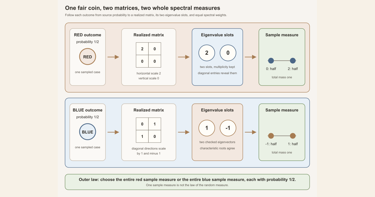
Let the sample space be
\[ \Omega=\{\mathrm{red},\mathrm{blue}\}. \]A sample space is the set of possible underlying outcomes. Declare every subset of \(\Omega\) to be an event , and assign the fair probability measure
\[ \mathbb P(\{\mathrm{red}\}) {} = \mathbb P(\{\mathrm{blue}\}) {} = \frac12. \]Define the matrix-valued rule \(X\) by
\[ X(\mathrm{red}) {} = R= \begin{bmatrix} 2&0\\ 0&0 \end{bmatrix}, \qquad X(\mathrm{blue}) {} = B= \begin{bmatrix} 0&1\\ 1&0 \end{bmatrix}. \]The function \(X\) is the random matrix. The ordinary matrix \(R\) or \(B\) seen after one coin toss is a realization, also called a sample value. One realization is not the whole random matrix, just as one coin toss is not the coin-tossing rule.
Check every coordinate before invoking probability
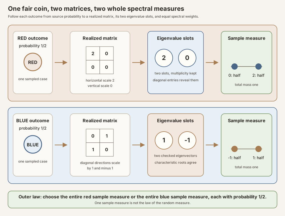
Write \(X_{ij}(\omega)=X(\omega)_{ij}\). In this example the four scalar coordinate functions have the following values:
| Entry map | At red | At blue |
|---|---|---|
| \(X_{00}\) | \(2\) | \(0\) |
| \(X_{01}\) | \(0\) | \(1\) |
| \(X_{10}\) | \(0\) | \(1\) |
| \(X_{11}\) | \(0\) | \(0\) |
Because every subset of the two-point source is measurable, the preimage of every scalar event is measurable. For example,
\[ \{\omega:X_{00}(\omega)\gt1\} {} = \{\mathrm{red}\}, \qquad \mathbb P\{X_{00}\gt1\} {} = \frac12. \]This one calculation already has the shape of a pushforward law: define a measurable target set, pull it back through the random object, and measure the resulting source event.
Check the red realization and its spectrum
An eigenvalue of a matrix \(H\) is a scalar \(\lambda\) for which some nonzero vector \(v\) satisfies \(Hv=\lambda v\). Such a vector is an eigenvector. The matrix \(R\) is diagonal. Its standard basis vectors satisfy
\[ R \begin{bmatrix}1\\0\end{bmatrix} {} = 2\begin{bmatrix}1\\0\end{bmatrix}, \qquad R \begin{bmatrix}0\\1\end{bmatrix} {} = 0\begin{bmatrix}0\\1\end{bmatrix}. \]Its two eigenvalue slots, counted with multiplicity, are therefore \(2\) and \(0\). Equivalently,
\[ \det(\lambda I-R)=\lambda(\lambda-2). \]Check the blue realization and its spectrum
The blue matrix swaps the two coordinates. The two diagonal directions obey
\[ B \begin{bmatrix}1\\1\end{bmatrix} {} = 1\begin{bmatrix}1\\1\end{bmatrix}, \qquad B \begin{bmatrix}1\\-1\end{bmatrix} {} = -1\begin{bmatrix}1\\-1\end{bmatrix}. \]Thus the blue eigenvalue slots are \(1\) and \(-1\). The characteristic polynomial confirms the same roots:
\[ \det(\lambda I-B)=\lambda^2-1=(\lambda-1)(\lambda+1). \]Both realizations are real symmetric, hence complex Hermitian. A Hermitian matrix equals its own conjugate transpose . Its finite eigenvalues are real, which is why Hermitian matrix models lead naturally to measures on the real line (Mathlib contributors).
Turn each realized spectrum into one measure
The empirical spectral measure places equal mass on every eigenvalue slot. Each realization here has two slots, so
\[ L_R=\frac12\delta_2+\frac12\delta_0, \qquad L_B=\frac12\delta_1+\frac12\delta_{-1}. \]The symbol \(\delta_x\) denotes the Dirac measure at \(x\): it puts one unit of mass at \(x\) and none elsewhere. Each \(L\) above has total mass one. It is one measure produced by one realized matrix.
Now repeat the outer coin experiment. The empirical spectral law is
\[ \mathcal Q {} = \frac12\delta_{L_R}+\frac12\delta_{L_B}. \]The atoms of \(\mathcal Q\) are whole measures, not real eigenvalues. With outer probability \(1/2\), a sample from \(\mathcal Q\) returns \(L_R\); with outer probability \(1/2\), it returns \(L_B\).
One average is not the law on measures
If we average the two sample measures, we obtain one measure on \(\mathbb R\):
\[ \overline L {} = \frac12L_R+\frac12L_B {} = \frac14\delta_2+ \frac14\delta_1+ \frac14\delta_0+ \frac14\delta_{-1}. \]The types tell us why \(\mathcal Q\) and \(\overline L\) are different:
| Object | Mathematical type | What one sample returns |
|---|---|---|
| \(X\) | \(\Omega\to\mathbb C^{2\times2}\) | one matrix |
| \(L_X\) | \(\Omega\to\operatorname{Measure}(\mathbb R)\) | one spectral measure |
| \(\mathcal Q\) | \(\operatorname{Measure}(\operatorname{Measure}(\mathbb R))\) | one whole spectral measure |
| \(\overline L\) | \(\operatorname{Measure}(\mathbb R)\) | one real location, if sampled |
The average forgets which eigenvalues arrived together. For example, under \(\mathcal Q\), eigenvalues \(2\) and \(0\) occur in the same matrix sample. The single measure \(\overline L\) retains their marginal masses but not that pairing.
This distinction is central to the repository’s typed-object ledger. A sample measure, its law on a space of measures, a bundled probability-valued law, and a Giry barycenter, which integrates the inner measures into one mean measure, are related constructions, not interchangeable names.
A nearby nonexample: equal spectra can hide different operators
Consider
\[ Z= \begin{bmatrix} 0&0\\ 0&0 \end{bmatrix}, \qquad N= \begin{bmatrix} 0&1\\ 0&0 \end{bmatrix}. \]Both characteristic polynomials are \(\lambda^2\), so both empirical spectral measures are \(\delta_0\). Yet \(Z\) kills every vector, while
\[ N \begin{bmatrix}0\\1\end{bmatrix} {} = \begin{bmatrix}1\\0\end{bmatrix}. \]The matrix \(N\) is nonzero, nilpotent because \(N^2=0\), and not Hermitian. This boundary teaches two rules:
- real eigenvalues do not imply Hermitian symmetry; and
- an empirical spectral measure does not determine the original matrix.
The blue realization is recovered from this nonexample by unnormalized Hermitian symmetrization:
\[ N+N^*=B. \]Symmetrization changes the spectrum and the geometry. It is a constructor, not a harmless relabeling.
The abstract climb, now that every object has a face
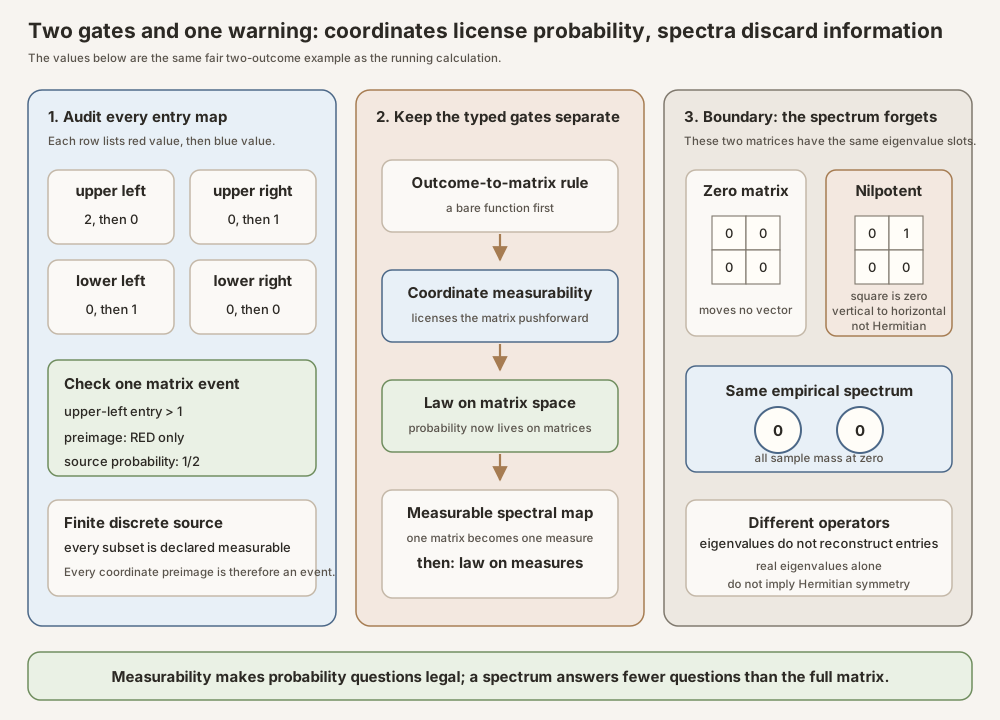
The running example instantiates five general layers.
1. Outcomes and measurable events
A measurable space \((\Omega,\mathcal F)\) consists of a set of outcomes and a collection \(\mathcal F\) of measurable events. A measure \(\mu\) assigns sizes to those events. When \(\mu(\Omega)=1\), it is a probability measure. These are the foundations for random elements and their laws (Kallenberg).
Our finite example uses \(\mathcal F=\mathcal P(\Omega)\), the collection of all subsets. In an uncountable sample space, not every subset is automatically declared measurable, so the measurability obligation becomes substantive.
2. A matrix-valued map
For index sets \(\iota\) and \(\kappa\), a matrix-valued map is
\[ X:\Omega\longrightarrow\mathbb K^{\iota\times\kappa}. \]The project’s base random matrix type is exactly this function. It deliberately stores neither a source measure nor a measurability proof. This makes the same function reusable under different measures and in deterministic arguments.
In standard probability language, the map becomes a matrix-valued random variable once it is measurable. A measurable function pulls every measurable target set back to a measurable source event.
3. Entrywise measurability
The project’s matrix space carries the product measurable structure generated by its entries, even before the index types are assumed finite. Under the project instance,
\[ X\text{ is measurable} \quad\Longleftrightarrow\quad \omega\longmapsto X(\omega)_{ij} \text{ is measurable for every }i,j. \]This theorem concerns visibility to a measure. It says nothing about whether different entries are independent. In a Hermitian matrix, lower-triangular entries are conjugates of upper-triangular entries, so they are deliberately dependent.
4. A realization and its spectral observable
Fixing \(\omega\) gives one ordinary matrix \(X(\omega)\). If that matrix is Hermitian, its finite eigenvalues are real. The ordered eigenvalue vector and the empirical spectral measure are deterministic functions of that one realization.
The project later proves that the ordered Hermitian eigenvalues are continuous, hence measurable, for its finite Frobenius geometry , the Euclidean geometry obtained by summing the squared magnitudes of all entries. This is a second measurability gate. Measurability of matrix entries does not make every nonlinear statistic automatically measurable; the statistic needs its own theorem.
5. Pushforward laws
Given a measurable map \(X\) and source measure \(\mu\), the pushforward law is
\[ \mathcal L_\mu(X)=X_*\mu. \]For every measurable matrix set \(D\),
\[ (X_*\mu)(D)=\mu(X^{-1}(D)). \]Applying the same construction to a measurable spectral-measure map produces a law whose points are measures. A probability distribution need not have a density; the running example is atomic, meaning its mass sits at finitely many individual points.
In Lean: from a bare carrier to Hermitian closure
The bare function is the first layer
X : NonlinearDynamics.Random.RandomMatrix Ω ι κ 𝕜Ωis the outcome type.ιandκare the row and column index types.𝕜is the scalar type, such asℝorℂ.Matrix ι κ 𝕜is Mathlib’s two-index function type for matrices.RandomMatrix Ω ι κ 𝕜unfolds toΩ → Matrix ι κ 𝕜.- The arrow
→is the same outcome-to-value arrow used on paper.
The checked definition is:
abbrev RandomMatrix
    (Ω : Type uΩ) (ι : Type uι) (κ : Type uκ) (𝕜 : Type u𝕜) :=
  Ω → Matrix ι κ 𝕜
An abbreviation introduces a project name without wrapping the function in a
new data constructor. Applying X to ω still gives the
realized matrix X ω directly.
The coordinate criterion is an equivalence
NonlinearDynamics.Random.RandomMatrix.measurable_iff_entries X : Measurable X ↔ ∀ i j, Measurable fun ω ↦ X ω i jMeasurable Xis the matrix-level claim.↔means both implications are proved.∀ i jmeans every row index and every column index.fun ω ↦ …constructs the scalar entry function.X ω i jfirst realizes the matrix atω, then reads rowiand columnj.- The theorem is about measurability only. No symbol here asserts independence, identical distribution, Gaussianity, or Hermitian symmetry.
The exact project proof is short because the matrix measurable structure was chosen entrywise:
theorem measurable_iff_entries (X : RandomMatrix Ω ι κ 𝕜) :
    Measurable X ↔ ∀ i j, Measurable fun ω ↦ X ω i j := by
  rw [measurable_comap_iff]
  change Measurable (fun ω i j ↦ X ω i j) ↔ _
  simp only [measurable_pi_iff]
Read the proof in three moves:
measurable_comap_iffunfolds the measurable structure pulled back from the curried function representation.changedisplays a matrix-valued function as a function of an outcome, row, and column.measurable_pi_iffreduces product-valued measurability to all coordinate maps.
This release-specific interface was checked against Mathlib 4.32.0. The exact pinned matrix source and pinned measurable-space source remain the implementation authority for the imported APIs (Mathlib contributors).
Build new measurable matrices entry by entry
The base module proves that the operations needed for finite matrix theory preserve measurability.
| Operation | Why each output entry is measurable | Extra finite gate |
|---|---|---|
| Transpose | read the input entry with swapped indices | none |
| Scalar map | compose one entry map with a measurable scalar function | none |
| Constant matrix | every entry is a constant function | none |
| Conjugate transpose | swap indices and take complex conjugation | none |
| Addition | add two measurable scalar functions | none |
| Multiplication | sum products of corresponding scalar functions | the shared index is finite |
For multiplication,
\[ (XY)_{ik}=\sum_jX_{ij}Y_{jk}. \]The theorem uses a finite sum over \(j\). It is not an infinite-dimensional operator theorem.
Unnormalized Hermitian symmetrization
For a square complex matrix-valued map, the project defines
\[ \operatorname{sym}(X)(\omega)=X(\omega)+X(\omega)^*. \]It proves this constructor measurable when \(X\) is measurable. Separately, it proves the result Hermitian at every outcome without needing a measurability assumption. The constructor is intentionally unnormalized. Some contexts use \((A+A^*)/2\), but that scaling would change future distributional and spectral formulas even though Hermiticity remains true.
NonlinearDynamics.Random.RandomMatrix.hermitianSymmetrization_isHermitian X ω : (NonlinearDynamics.Random.RandomMatrix.hermitianSymmetrization X ω).IsHermitianhermitianSymmetrization X ωapplies the constructor and then realizes it atω..IsHermitianis the matrix property that the conjugate transpose equals the matrix.- The explicit
ωmakes the statement pointwise. - The later almost-everywhere theorem uses
Filter.Eventually.of_forallto weaken this everywhere statement.
Pinned Mathlib’s Hermitian algebra supplies the matrix property and closure lemmas used here (Mathlib contributors).
Try the exact base declarations in the repository
Full project check: pinned project plus Mathlib. A learner can create a temporary project probe with:
import NonlinearDynamics.Random.RandomMatrices.Basic

#print NonlinearDynamics.Random.RandomMatrix
#check NonlinearDynamics.Random.RandomMatrix.measurable_iff_entries
#check NonlinearDynamics.Random.RandomMatrix.measurable_entry
#check NonlinearDynamics.Random.RandomMatrix.measurable_mul
#check NonlinearDynamics.Random.RandomMatrix.hermitianSymmetrization
#check NonlinearDynamics.Random.RandomMatrix.hermitianSymmetrization_isHermitian
#check NonlinearDynamics.Random.RandomMatrix.hermitianSymmetrization_isHermitianAE
#print unfolds the project abbreviation. Each
#check invokes the pinned elaborator and displays the exact type
of a checked declaration. Running the generated full project command below checks the
authoritative module; the temporary probe only requests declaration types.
cd formalization
lake env lean -DwarningAsError=true NonlinearDynamics/Random/RandomMatrices/Basic.lean
Resource note: this exact file uses the repository's
pinned Lean and Mathlib dependencies. Initial project setup can require
substantial disk space and build time. For a lightweight first step on
macOS or Linux, use the page's standalone Lean-core or Std
tutorial.
In Lean: from one Hermitian matrix to a random spectral law
Give one matrix a finite empirical measure
For an intrinsic \(n\)-by-\(n\) Hermitian matrix \(H\), let
\[ \lambda_0(H)\geq\lambda_1(H)\geq\cdots\geq\lambda_{n-1}(H) \]be its real eigenvalues with multiplicity. The spectral counting measure is
\[ \kappa_H=\sum_{i=0}^{n-1}\delta_{\lambda_i(H)}. \]Its total mass is \(n\). The empirical spectral measure is
\[ L_H=\frac1n\kappa_H \]when \(n\gt0\). Repeated eigenvalues contribute repeated atoms; replacing the vector by a set of distinct roots would lose multiplicity and produce the wrong trace moments.
Viewing each real integration variable as a complex number, the first two counting-measure moments recover the ordinary complex matrix traces:
\[ \int x\,d\kappa_H(x)=\operatorname{Tr}(H), \qquad \int x^2\,d\kappa_H(x)=\operatorname{Tr}(H^2). \]The empirical moments divide these by \(n\) in positive dimension. In the running example,
| Realization | First empirical moment | Second empirical moment |
|---|---|---|
| \(R\) with slots \(2,0\) | \((2+0)/2=1\) | \((2^2+0^2)/2=2\) |
| \(B\) with slots \(1,-1\) | \((1-1)/2=0\) | \((1^2+(-1)^2)/2=1\) |
At dimension zero, the finite sum has no atoms. The repository deliberately defines both the counting measure and empirical measure to be the zero measure. The empirical measure is therefore zero or probabilistic in all dimensions, and a bundled probability-measure wrapper appears only in positive dimension. No fake eigenvalue is inserted at zero.
NonlinearDynamics.Random.RandomMatrix.spectralCountingMeasure H; NonlinearDynamics.Random.RandomMatrix.empiricalSpectralMeasure HHis an intrinsicHermitianEuclidean nvalue.orderedHermitianEigenvalues H iis the real eigenvalue in sloti : Fin n.spectralCountingMeasure Hhas typeMeasure ℝand adds one Dirac mass per slot.empiricalSpectralMeasure Halso has typeMeasure ℝ; it applies the project’s zero-aware normalization.- Neither expression is a probability law on matrices or on measures. Each is
a deterministic measure attached to one matrix
H.
Push a matrix law to a law on spectral measures
The matrix-law layer makes measurability explicit:
noncomputable def law (X : RandomMatrix Ω ι ι ℂ) (_hX : Measurable X)
    (μ : Measure Ω) : Measure (Matrix ι ι ℂ) :=
  Measure.map X μ
The keyword noncomputable permits a classical mathematical
definition that Lean is not promising to execute as a program. It does not
weaken the proposition proved about the resulting measure.
The proof argument _hX is semantically important even though the
value of Measure.map does not store it. Mathlib’s map operation is
total and has fallback behavior outside the
almost-everywhere
measurable case. The
project name law therefore demands evidence that the standard
pushforward interpretation is licensed.
NonlinearDynamics.Random.RandomMatrix.law X hX μ; NonlinearDynamics.Random.RandomMatrix.law_apply X hX μ hDhX : Measurable Xis the gate that licenses the law.μ : Measure Ωis the source measure.RandomMatrix.law X hX μhas typeMeasure (Matrix ι ι ℂ).Dis a set of matrices andhD : MeasurableSet Dproves that it is a legal target event.law_applystates the exact preimage evaluation rule.
At the later finite Gaussian unitary ensemble (GUE) layer, the repository has proved that the empirical-spectral-measure observable is measurable and names its pushforward law:
NonlinearDynamics.Random.GUE.empiricalSpectralLaw n = (NonlinearDynamics.Random.GUE.intrinsicLaw n).map NonlinearDynamics.Random.RandomMatrix.empiricalSpectralMeasureGUE.intrinsicLaw nis a probability law on intrinsic Hermitian matrices.RandomMatrix.empiricalSpectralMeasuremaps one matrix to oneMeasure ℝ..mappushes the matrix law through that measurable observable.- The result has type
Measure (Measure ℝ). The outer measure is the random law; each point in its carrier is an inner spectral measure. - This named project law is not the fair-coin law \(\mathcal Q\) computed above. The coin model is a finite teaching analogue of the same typed path.
Run the finite model locally with Lean and Std
This first worksheet is deliberately tiny. It imports only Lean’s
Std library, uses two fixed integer matrices, and performs bounded
list computations. It does not import Mathlib, open the repository’s Lake
project, download a cache, or prove measure-theoretic measurability.
Create a scratch directory outside formalization/. Save the
following as CoinMatrixTutorial.lean:
import Std

inductive Outcome where
  | red
  | blue
deriving Repr, DecidableEq

structure Matrix2 where
  a00 : Int
  a01 : Int
  a10 : Int
  a11 : Int
deriving Repr, DecidableEq

abbrev Vec2 := Int × Int

def outcomeLabel : Outcome → String
  | .red => "red"
  | .blue => "blue"

def sampleMatrix : Outcome → Matrix2
  | .red => ⟨2, 0, 0, 0⟩
  | .blue => ⟨0, 1, 1, 0⟩

def entries (A : Matrix2) : Int × Int × Int × Int :=
  (A.a00, A.a01, A.a10, A.a11)

def mulVec (A : Matrix2) (v : Vec2) : Vec2 :=
  (A.a00 * v.1 + A.a01 * v.2,
   A.a10 * v.1 + A.a11 * v.2)

def scaleVec (lambda : Int) (v : Vec2) : Vec2 :=
  (lambda * v.1, lambda * v.2)

structure Eigenpair where
  value : Int
  vector : Vec2
deriving Repr, DecidableEq

def eigenpairs : Outcome → List Eigenpair
  | .red => [⟨2, (1, 0)⟩, ⟨0, (0, 1)⟩]
  | .blue => [⟨1, (1, 1)⟩, ⟨-1, (1, -1)⟩]

def eigenpairOK (A : Matrix2) (pair : Eigenpair) : Bool :=
  decide (mulVec A pair.vector = scaleVec pair.value pair.vector)

def spectrum (omega : Outcome) : List Int :=
  (eigenpairs omega).map (fun pair => pair.value)

def spectralCertificate (omega : Outcome) : Bool :=
  (eigenpairs omega).all (eigenpairOK (sampleMatrix omega))

def outcomes : List Outcome := [.red, .blue]

def largeFirstEntryPreimage : List String :=
  (outcomes.filter (fun omega => decide ((sampleMatrix omega).a00 > 1))).map
    outcomeLabel

def quarterMass (x : Int) : Nat :=
  outcomes.foldl (fun total omega => total + (spectrum omega).count x) 0

def meanMassLedger : List (Int × Nat) :=
  ([-1, 0, 1, 2] : List Int).map (fun x => (x, quarterMass x))

#eval outcomes.map (fun omega =>
  (outcomeLabel omega, entries (sampleMatrix omega)))
#eval outcomes.map (fun omega => (outcomeLabel omega, spectrum omega))
#eval outcomes.map (fun omega =>
  (outcomeLabel omega, spectralCertificate omega))
#eval largeFirstEntryPreimage
#eval meanMassLedger

example : spectralCertificate .red = true := by decide
example : spectralCertificate .blue = true := by decide
example : largeFirstEntryPreimage = ["red"] := by decide
example : meanMassLedger = [(-1, 1), (0, 1), (1, 1), (2, 1)] := by decide
Open a terminal in that scratch directory and type:
source "$HOME/.elan/env"
elan run leanprover/lean4:v4.32.0 lean CoinMatrixTutorial.lean
This exact worksheet was executed successfully with Lean 4.32.0. It printed:
[("red", 2, 0, 0, 0), ("blue", 0, 1, 1, 0)]
[("red", [2, 0]), ("blue", [1, -1])]
[("red", true), ("blue", true)]
["red"]
[(-1, 1), (0, 1), (1, 1), (2, 1)]
Read the output in order:
- the first line shows the two realized matrices in row-major entry order;
- the second shows the two eigenvalue-slot lists;
- the third verifies all four displayed eigenvector equations;
- the fourth computes the preimage of the upper-left-entry event; and
- the fifth records the averaged spectral mass in quarter-units, so each listed eigenvalue has mass \(1/4\).
The four example declarations are kernel-checked proofs of the
same finite claims. This worksheet checks the arithmetic and type
separation of the toy model. It does not establish the general spectral theorem, matrix
measurability, pushforward law, or project declarations below.
Try the exact spectral-law declarations in the repository
Full project check: later project modules plus Mathlib. Install the repository’s pinned dependencies, then type this probe:
import NonlinearDynamics.Random.RandomMatrices.GaussianUnitaryEnsembleSpectrum

#check NonlinearDynamics.Random.RandomMatrix.orderedHermitianEigenvalues
#check NonlinearDynamics.Random.RandomMatrix.spectralCountingMeasure
#check NonlinearDynamics.Random.RandomMatrix.empiricalSpectralMeasure
#check NonlinearDynamics.Random.RandomMatrix.empiricalSpectralMeasure_zero
#check NonlinearDynamics.Random.RandomMatrix.measurable_empiricalSpectralMeasure
#check NonlinearDynamics.Random.GUE.empiricalSpectralLaw
#check NonlinearDynamics.Random.GUE.empiricalSpectralLaw_zero
#check NonlinearDynamics.Random.GUE.meanEmpiricalSpectralMeasure
These names span the deterministic sample spectrum, its zero-dimensional boundary, measurability of the measure-valued observable, the outer finite GUE law, and its mean measure. The full project command below checks the full imported leaf and may require substantial disk space and memory.
cd formalization
lake env lean -DwarningAsError=true NonlinearDynamics/Random/RandomMatrices/GaussianUnitaryEnsembleSpectrum.lean
Resource note: this exact file uses the repository's
pinned Lean and Mathlib dependencies. Initial project setup can require
substantial disk space and build time. For a lightweight first step on
macOS or Linux, use the page's standalone Lean-core or Std
tutorial.
What the repository has checked, and what it has not
The page’s primary module,
NonlinearDynamics.Random.RandomMatrices.Basic, proves only the
entrywise measurable foundation and its finite algebraic closure. Later
modules now add substantial finite theory:
| Layer | Checked repository contribution |
|---|---|
| Matrix carrier | outcome-to-matrix functions and the entrywise measurable structure |
| Hermitian structure | pointwise and almost-everywhere Hermiticity, bundled measurable Hermitian matrices, and congruence |
| Matrix law | measurable pushforwards, probability preservation, Dirac rules, and unitary-invariance interfaces |
| Finite GUE | exact Wigner-scaled coordinate law, ambient matrix law, zero-dimensional Dirac boundary, and unitary invariance |
| Finite observables | measurable trace powers and the first two exact integrable finite GUE trace moments |
| Finite spectrum | ordered real Hermitian eigenvalues, counting and empirical measures, perturbation continuity, and measurability |
| Spectral law | the finite GUE law on empirical spectral measures, its mean measure, and first two normalized expected sample moments |
Here GUE means Gaussian unitary ensemble. The project’s convention is
Wigner scaled: diagonal variance \(1/n\), off-diagonal real and imaginary
variances \(1/(2n)\), ordinary matrix trace, and an order-one spectrum in
positive dimension. That normalization belongs to the GUE modules, not to the
bare RandomMatrix definition. Standard references explain why
normalization ledgers and symmetry classes matter
(Tao; Anderson, Guionnet, and Zeitouni).
For positive dimension, the complete convention ledger is:
| Convention field | This project’s finite GUE choice |
|---|---|
| Dimension | \(n\times n\), with a separate explicit Dirac policy at \(n=0\) |
| Diagonal coordinates | independent centered real Gaussians of variance \(1/n\) |
| Strict-upper coordinates | independent complex coordinates whose real and imaginary parts are independent centered Gaussians, each of variance \(1/(2n)\) |
| Lower triangle | conjugate reflection of the strict upper triangle, not new independent data |
| Density exponent | the associated classical convention is proportional to \(\exp[-n\operatorname{Tr}(H^2)/2]\); the repository has not proved a density theorem |
| Spectral scale | the \(n^{-1/2}\) scale is already built into the entries, producing an order-one spectrum |
| Trace | Matrix.trace is ordinary; empirical moments introduce the factor \(n^{-1}\) separately |
The density row records the convention needed to compare literature formulas. It is explanatory context, not a checked density identity.
The checked unitary invariance statement is law-level symmetry: pushing the finite GUE matrix law through \(H\mapsto UHU^*\) leaves that law unchanged for every unitary \(U\). It is not pointwise equality \(UHU^*=H\).
The repository does not yet prove:
- a Hermitian-space or joint-eigenvalue density formula;
- the semicircle law or any large-dimension spectral limit;
- local spacing universality, edge statistics, or Tracy-Widom laws;
- a Gaussian orthogonal or symplectic ensemble;
- that an empirical spectral measure determines its matrix;
- that a random Jacobian belongs to GUE;
- a physical quantum-chaos conclusion from the finite GUE construction; or
- any result merely because the running two-outcome worksheet computed it.
The first four absences are later random-matrix work. The remaining four are claim boundaries: spectra discard information, modeling assumptions must be stated, and a pedagogical computation is not a project theorem.
Why physicists care, without skipping the assumptions
Hermitian random matrices became central in mathematical physics because Hermitian operators model finite quantum observables and have real energy levels. Wigner used random-matrix ideas to study the statistics of complex nuclear spectra, and Dyson organized the orthogonal, unitary, and symplectic symmetry classes (Wigner, 1955; Dyson, 1962; Dyson, Threefold Way).
That history motivates an ensemble. It does not prove that a particular Hamiltonian has independent Gaussian coordinates or that one finite sample already exhibits a universal limit. The project therefore formalizes the finite probability object and its normalization before asking asymptotic or physical questions.
Two bridges back to nonlinear dynamics
Random Jacobians
The derivative of a random or uncertain dynamical system can be a random matrix. Its action on perturbation vectors and its singular values can encode one-step growth. Eigenvalues of one fixed linearization answer a narrower question and can miss transient growth for a nonnormal matrix, one that does not commute with its conjugate transpose. The nilpotent boundary above already shows that eigenvalues can miss operator action.
The measurable-matrix layer can carry such Jacobians without assuming they are Gaussian, Hermitian, independent, or identically distributed.
Matrix cocycles
Linearization along an orbit produces ordered products
\[ A_{t-1}\cdots A_1A_0. \]A base transformation and generator can organize these matrices into a one-sided random matrix cocycle . Long-time norm growth then leads toward Lyapunov exponents, asymptotic exponential growth rates, under additional integrability and ergodicity hypotheses. The finite measurable multiplication theorem is one early ingredient, not a Lyapunov theorem by itself.
Exercises: use the same example until every layer is yours
- Preimage. Compute the source event where the lower-left entry equals one. What probability does it have?
- Realization. Multiply both \(R\) and \(B\) by \((1,2)\). Which output belongs to each outcome?
- Eigenpairs. Verify the four eigenvector equations without using the characteristic polynomial.
- Characteristic roots. Expand both determinants \(\det(\lambda I-R)\) and \(\det(\lambda I-B)\).
- Sample moments. Recompute the first two empirical moments in the table.
- Outer event. Let \(C\) be the set of empirical measures assigning positive mass to \(\{2\}\). Compute \(\mathcal Q(C)\).
- Law versus mean. Construct a different law on measures whose mean is \(\overline L\). Explain what sample-to-sample information changes.
- Boundary. Verify \(N^2=0\), \(N\ne0\), and \(N\ne N^*\).
- Symmetrization. Compute \((N+N^*)/2\). How do its eigenvalues compare with the unnormalized blue matrix \(B\)?
- Lean tokens. In the local worksheet, change the red diagonal entry from \(2\) to \(3\). Update its eigenpair certificate, spectrum, event preimage, and mass ledger together.
- Resource boundary. Explain why the
Stdstandalone tutorial is small while the two full project checks load the repository’s pinned Mathlib dependencies. - Research boundary. Name one additional theorem needed before a finite spectral law can support a large-dimension universality claim.
Where to continue
- Start with Random matrix for a compact account of the carrier, realization, measurability, and law distinction.
- Continue to Finite Hermitian Matrices from Coordinates for direct assembly from nonredundant coordinates.
- Use Finite Hermitian Spectra and Empirical Measures for the ordered spectrum, multiplicity, zero-dimensional policy, and deterministic measure layer.
- Then read Hermitian Spectral Perturbation, Continuity, and Measurability for the theorem that opens the spectral pushforward gate.
- Finish the finite path with Finite Gaussian Unitary Ensemble Empirical Spectral Laws and Normalized Moments.
References
Mathlib contributors. Measurable spaces and measurable functions, Mathlib 4 documentation. Accessed 2026-07-20. This is the implementation-level source for Lean’s measurable-space and measurable-function interfaces.
Mathlib contributors.
Mathlib 4.32.0 release,
commit 81a5d257c8e410db227a6665ed08f64fea08e997. This is the exact dependency
release against which the Lean declarations in this chapter were checked.
Mathlib contributors.
Hermitian matrices,
Mathlib 4 documentation. Accessed 2026-07-20. This documents
Matrix.IsHermitian and the algebraic closure lemmas used by the
project.
Mathlib contributors. Spectral theory of matrices, Mathlib 4 documentation. Accessed 2026-07-20. This documents the finite Hermitian spectral infrastructure consumed by the later project modules.
Terence Tao. Topics in Random Matrix Theory, Graduate Studies in Mathematics 132, American Mathematical Society, 2012. The author’s book page links an online draft, lecture notes, and errata.
Olav Kallenberg. Foundations of Modern Probability, third edition, Probability Theory and Stochastic Modelling 99, Springer, 2021. This is a standard source for measurable random elements, laws, product spaces, independence, and almost-everywhere reasoning.
Greg W. Anderson, Alice Guionnet, and Ofer Zeitouni. An Introduction to Random Matrices, Cambridge Studies in Advanced Mathematics 118, Cambridge University Press, 2010. This is a standard systematic source for real and complex Wigner matrices, Gaussian ensembles, and asymptotic spectral theory.
Eugene P. Wigner. Characteristic Vectors of Bordered Matrices With Infinite Dimensions, Annals of Mathematics 62(3), 548-564, 1955. This is cited for historical context on random-matrix models of complex spectra, not as a source for the Lean implementation.
Freeman J. Dyson. Statistical Theory of the Energy Levels of Complex Systems. I, Journal of Mathematical Physics 3, 140-156, 1962. This is cited for the symmetry-class framing that connects orthogonal, unitary, and symplectic ensembles to physical invariances.
Freeman J. Dyson. The Threefold Way: Algebraic Structure of Symmetry Groups and Ensembles in Quantum Mechanics, Journal of Mathematical Physics 3(6), 1199-1215, 1962. This is the original three-class symmetry analysis, not the broader later tenfold classification.