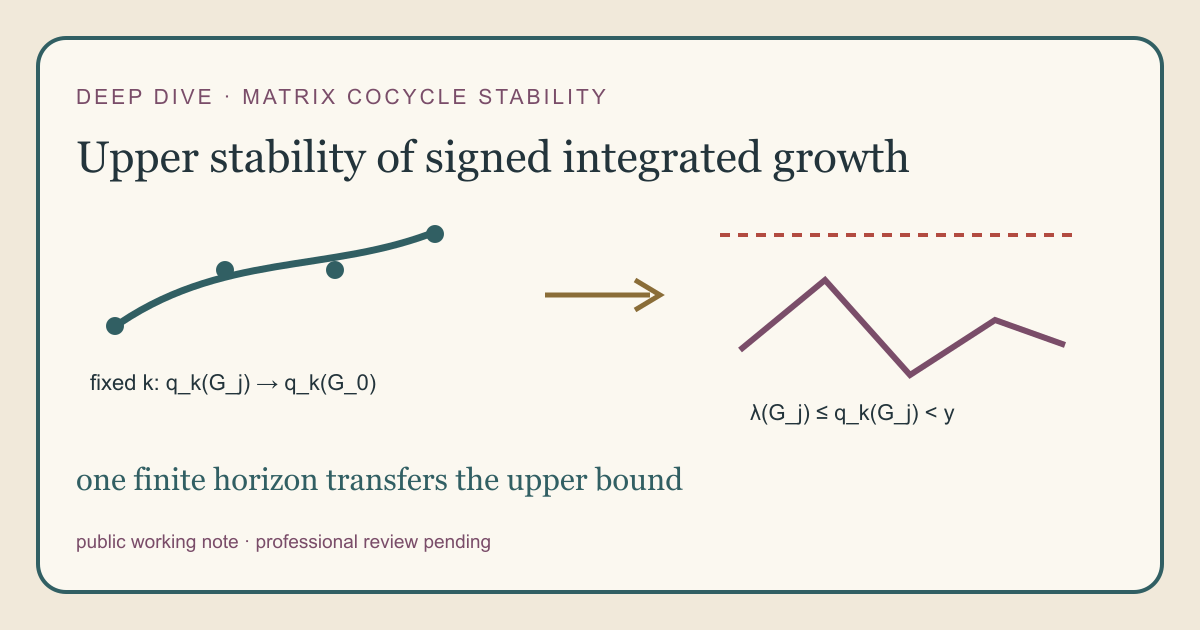
A calculation before the general statement
On the one-point probability space with identity base, choose \(G_j=[e^{2+1/(j+1)}]\) and \(G_0=[e^2]\). Every positive horizon \(k\) has
\[ \frac1k\log\lVert G_j^k\rVert=2+\frac1{j+1}, \qquad \frac1k\log\lVert G_0^k\rVert=2. \]The exact rates converge from above to \(2\). All generators and inverses have common norm bounds. Replacing \(2\) with a negative number gives the same calculation in the contracting regime.
This example makes three roles visible. The perturbation index \(j\) varies the generator. The horizon \(k\) measures cocycle time. The output \(\lambda(G_j)\) is a deterministic number obtained after integration and a long-horizon Fekete limit. These indices and operations cannot be exchanged without justification.
The theorem in mathematical language
Fix a probability space \((\Omega,\mu)\), a measure-preserving map \(T:\Omega\to\Omega\), and a finite matrix dimension. Let \(G_j\) and \(G_0\) be measurable matrix-valued functions such that:
- \(G_j(\omega)\) is invertible for every \(j,\omega\);
- \(\lVert G_j(\omega)\rVert\le M\) for one common \(M\);
- \(\lVert G_j(\omega)^{-1}\rVert\le K\) for one common \(K\); and
- \(G_j\to G_0\) uniformly on \(\Omega\).
Then
\[ \limsup_{j\to\infty}\lambda(G_j)\le\lambda(G_0), \]where \(\lambda(G)\) is the signed integrated real-log Fekete rate from RMT-35.
Layer one: finite products
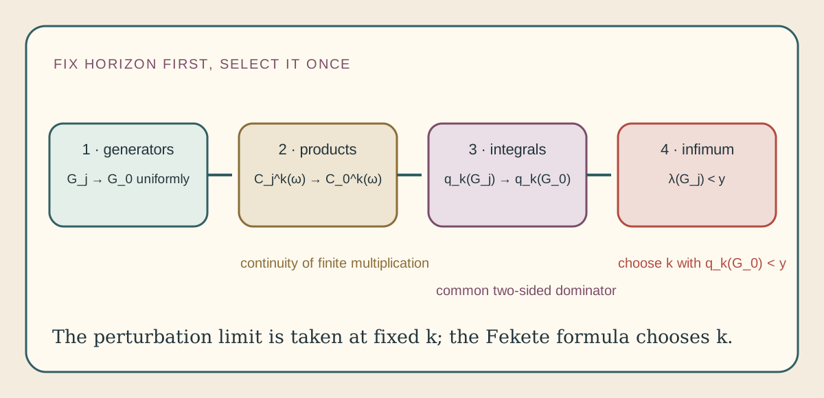
For fixed \(k\),
\[ C_j^k(\omega)= G_j(T^{k-1}\omega)\cdots G_j(\omega). \]There are only \(k\) factors. Uniform convergence supplies convergence at
every displayed orbit point, and continuity of multiplication transfers it to
the product. The theorem
tendsto_value_of_tendstoUniformly proves this by induction on \(k\).
Pointwise invertibility matters before taking the logarithm. It guarantees \(\lVert C_0^k(\omega)\rVert\ne0\), which is the continuity domain needed for \(\log\lVert\cdot\rVert\).
Layer two: a two-sided envelope
The forward bound gives
\[ \log\lVert C_j^k(\omega)\rVert\le k\log^+M. \]The inverse product gives the lower estimate
\[ -k\log^+K\le\log\lVert C_j^k(\omega)\rVert. \]Together,
\[ \left|\log\lVert C_j^k(\omega)\rVert\right| \le k(\log^+M+\log^+K). \]The right side depends on \(k\) but not on \(j\) or \(\omega\). For each fixed horizon it is integrable on the probability space, so dominated convergence transfers the finite-horizon signed integrals.
The inverse bound is essential for this proof. A forward bound alone controls large positive log norms but does not control near-singular contraction and large negative log norms.
abs_realLogNormObservable_le G hT k ω\n\ntendsto_integratedRealLogNorm_of_tendstoUniformly hT hG kUniformlyBoundedInvertibleGenerator.Layer three: the infimum witness
Write
\[ q_k(G)=\frac1k\int\log\lVert C_G^k\rVert\,d\mu. \]RMT-35 proves
\[ \lambda(G)=\inf_{k\ge1}q_k(G). \]Choose \(y\gt\lambda(G_0)\). By convergence of \(q_k(G_0)\) to its Fekete rate, some positive \(k\) satisfies \(q_k(G_0)\lt y\). Layer two gives \(q_k(G_j)\lt y\) eventually. Finally,
\[ \lambda(G_j)\le q_k(G_j)\lt y. \]The proof does not need convergence to be uniform in the horizon \(k\). Selecting one horizon before transferring it is the key economy.
In Lean
theorem eventually_integratedRealLogGrowthRate_lt\n [IsProbabilityMeasure μ]\n (hT : MeasurePreserving T μ μ)\n (hG : TendstoUniformly\n+ (fun n ↦ (G n : Ω → Matrix ι ι ℂ)) G₀ atTop)\n+ (hy : G₀.integratedRealLogGrowthRate hT < y) :\n+ ∀ᶠ n in atTop,\n+ (G n).integratedRealLogGrowthRate hT < yhy chooses the strict upper threshold. The conclusion is an eventual
statement in the perturbation index. MeasurePreserving fixes both the base
and the measure throughout the sequence.cd formalization
lake env lean -DwarningAsError=true NonlinearDynamics/Random/RandomCocycles/GrowthRateStability.leanResource note: this exact file uses the repository's
pinned Lean and Mathlib dependencies. Initial project setup can require
substantial disk space and build time. For a lightweight first step on
macOS or Linux, use the page's standalone Lean-core or Std
tutorial.
Which stochastic-stability question?
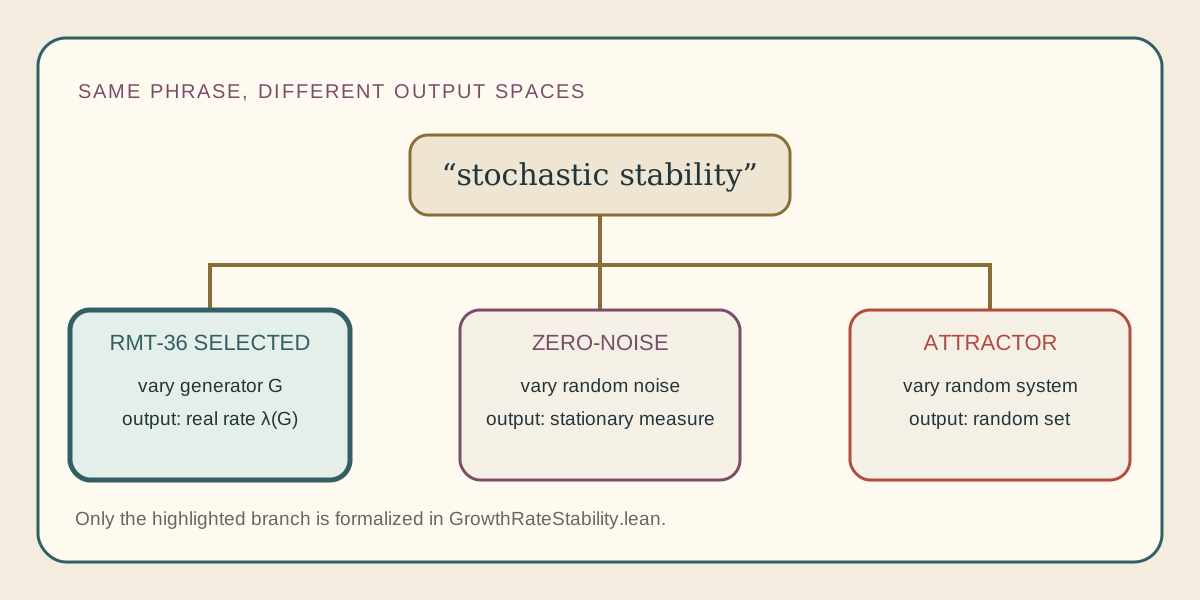
The selected branch varies a generator and outputs one real number. In zero-noise stochastic stability, the perturbation parameter often changes a Markov process or random perturbation and the output is a stationary measure. In random-attractor stability, the output is a random set compared using a set distance. Sharing a phrase does not identify these mathematical objects.
What upper semicontinuity permits
Upper semicontinuity prohibits late rates from remaining above \(\lambda(G_0)+\varepsilon\). It permits lower rates. The Fekete formula explains the asymmetry: an infimum has readily transferable upper witnesses, while lower bounds must control every horizon at once or use additional structure.
The result therefore supplies no lower semicontinuity, full continuity, modulus of continuity, or convergence rate. It also does not vary the base or measure, admit a singular limit, identify the remaining Lyapunov spectrum, or control invariant splittings.
Related trail markers
- Upper semicontinuity
- Integrated real-log growth rate
- Probability measure
- Measure-preserving transformation
- Upper Stability of Signed Cocycle Growth in Lean
References
- J. F. C. Kingman, “The Ergodic Theory of Subadditive Stochastic Processes,” Journal of the Royal Statistical Society: Series B 30(3), 499–510 (1968), doi:10.1111/j.2517-6161.1968.tb00749.x.
- J. Bochi, “Genericity of zero Lyapunov exponents,” Ergodic Theory and Dynamical Systems 22(6), 1667–1696 (2002), doi:10.1017/S0143385702001165.
- L. Backes, A. Brown, and C. Butler, “Continuity of Lyapunov exponents for cocycles with invariant holonomies,” Journal of Modern Dynamics 12, 223–260 (2018), doi:10.3934/jmd.2018009.
- M. Viana and J. Yang, “Continuity of Lyapunov exponents in the \(C^0\) topology,” Israel Journal of Mathematics 229, 461–485 (2019), doi:10.1007/s11856-018-1809-7.
- J. F. Alves, V. Araújo, and C. H. Vásquez, “Stochastic stability of diffeomorphisms with dominated splitting,” arXiv:math/0404160.
- J. C. Robinson, “Stability of random attractors under perturbation and approximation,” Journal of Differential Equations 186(2), 652–669 (2002), doi:10.1016/S0022-0396(02)00038-4.