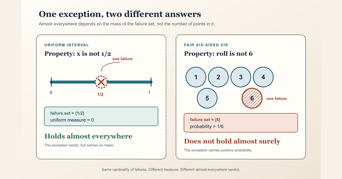
A property holds almost everywhere with respect to a measure \(\mu\) when the set of points where it fails has \(\mu\)-measure zero. Analysts abbreviate this as a.e. The word “almost” does real work: exceptions may exist. What matters is the amount of measure they carry.
See it with one real exception
Use the interval \(\Omega=[0,1]\) with the uniform probability measure. For an interval \([a,b]\subseteq[0,1]\), this measure assigns probability \(b-a\). Consider the property
\[ P(x):\quad x\ne \frac12. \]There is exactly one failure: \(P(1/2)\) is false. Its failure set is
\[ N=\left\{\frac12\right\}. \]A single point has length, and therefore uniform measure, zero:
\[ \mu(N)=\mu\left(\left\{\frac12\right\}\right)=0. \]So \(x\ne 1/2\) holds for \(\mu\)-almost every \(x\in[0,1]\), even though it does not hold for every \(x\). This is the smallest useful example because the exception is visible and the answer can be checked exactly.
Why the same-looking exception can fail
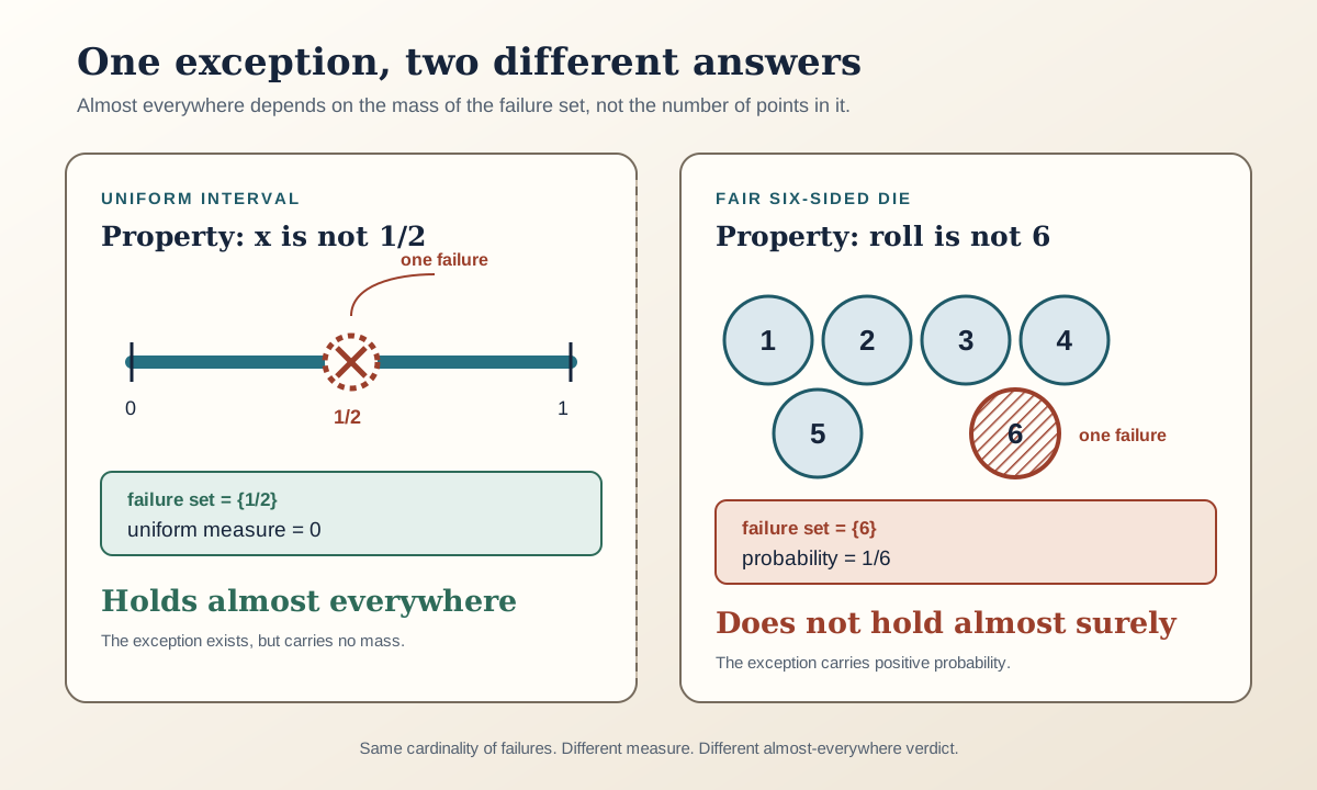
Now roll a fair six-sided die and let \(Q(k)\) mean \(k\ne6\). The failure set is again a singleton, \(\{6\}\), but the measure has changed:
\[ \mathbb P(\{6\})=\frac16\ne0. \]Therefore \(Q\) does not hold almost surely. On a finite probability space where every outcome has positive probability, the only null set is the empty set. “One exceptional point” is not enough information; the measure is part of the statement.
The definition on paper
Let \(\Omega\) be a set, let \(\mu\) be a measure on it, and let \(P:\Omega\to\mathrm{Prop}\) be a property. Define the failure set
\[ F_P=\{\omega\in\Omega:\neg P(\omega)\}. \]Then
\[ P(\omega)\text{ for }\mu\text{-almost every }\omega \quad\Longleftrightarrow\quad \mu(F_P)=0. \]Equivalently, there is a null set \(N\) such that \(P(\omega)\) holds at every \(\omega\notin N\). The null set need not be unique: any larger null set that contains all failures works as well.
For two functions \(f,g:\Omega\to S\), analysts write
\[ f=g\quad\mu\text{-a.e.} \]when the equality \(f(\omega)=g(\omega)\) holds outside a null set. This is weaker than equality as functions. Two representatives may disagree at \(1/2\) in the interval example and still be equal almost everywhere.
In Lean: read the quantifier, not just the symbols
∀ᵐ ω ∂μ, P ω∀ᵐis the almost-everywhere quantifier, not Lean’s ordinary∀.ωis the bound outcome; it is local to the statement.∂μsays which measure determines which exceptions may be ignored.P ωis the property tested at that outcome.- The whole expression is a proposition. It can be used as an assumption, theorem conclusion, or field in a larger definition.
The notation is filter-based: Lean interprets ∀ᵐ ω ∂μ, P ω as
saying that the set of outcomes satisfying \(P\) belongs to the
almost-everywhere filter generated by \(\mu\). The filter interface lets a
proof combine several almost-everywhere facts without repeatedly rebuilding
unions of null sets.
Small standalone tutorial: count the die failures
The continuous interval example needs measure theory, but the page’s fair-die
counterexample has a finite check that uses only Std. Because every
die face has positive probability, a property holds almost everywhere on this
finite model exactly when its failure list is empty. Create
/tmp/AlmostEverywhereDie.lean with these contents:
import Std

namespace AlmostEverywhereDie

def dieFaces : List Nat :=
  (List.range 6).map (fun k => k + 1)

def notSix (face : Nat) : Bool :=
  decide (face ≠ 6)

def failureFaces (P : Nat → Bool) : List Nat :=
  dieFaces.filter (fun face => !(P face))

def finiteAlmostEverywhere (P : Nat → Bool) : Bool :=
  failureFaces P == []

#eval failureFaces notSix
#eval finiteAlmostEverywhere notSix

example : failureFaces notSix = [6] := by decide
example : finiteAlmostEverywhere notSix = false := by decide

end AlmostEverywhereDie
From any directory on a normal macOS or Linux machine with the pinned compiler, type exactly:
source "$HOME/.elan/env"
elan run leanprover/lean4:v4.32.0 lean /tmp/AlmostEverywhereDie.lean
This exact worksheet was executed successfully with Lean 4.32.0 while repairing this page. It printed:
[6]
false
The first line finds the one failure. The second line confirms that this failure is not ignorable in the fair-die model. This bounded tutorial does not import Mathlib and does not test the interval’s zero-measure singleton.
Exact project and Mathlib interface
The project uses the notation in the checked definition
def IsHermitianAE (X : RandomMatrix Ω ι ι ℂ) (μ : Measure Ω) : Prop :=
  ∀ᵐ ω ∂μ, (X ω).IsHermitian
Read it aloud as: “with respect to \(\mu\), the realized matrix \(X(\omega)\) is Hermitian for almost every outcome \(\omega\).” The function \(X\), its realized value \(X(\omega)\), the Hermitian predicate, and the measure are all visible in the type.
Here is a complete small worksheet a human can type. Its final example uses the same pointwise-to-almost-everywhere proof step as the checked project theorem for Hermitian symmetrization.
import NonlinearDynamics.Random.RandomMatrices.Basic

open NonlinearDynamics.Random

#check RandomMatrix.IsHermitianAE
#check RandomMatrix.hermitianSymmetrization_isHermitianAE

example {Ω : Type*} [MeasurableSpace Ω] (μ : Measure Ω)
    (P : Ω → Prop) (hP : ∀ ω, P ω) : ∀ᵐ ω ∂μ, P ω :=
  Filter.Eventually.of_forall hP
How a human types Ω →
In a Lean-aware editor, type \Omega and then press Space to
produce Ω. Type \to and then press Space to produce
→. Thus a human can enter Ω → Prop as
\Omega, Space, \to, Space, Prop.
Unicode is convenient, not mandatory. Without input expansion, use an ASCII name and arrow:
variable (Omega : Type*)
#check Omega -> Omega
Lean reads Omega -> Omega as the same kind of function type as
Ω → Ω; only the variable’s spelling differs.
The example is pedagogical; the two #check lines
point at declarations in the named project file.
Filter.Eventually.of_forall performs the safe one-way conversion:
if there are no exceptions, then certainly all failures are confined to a null
set.
The exact checked source is
formalization/NonlinearDynamics/Random/RandomMatrices/Basic.lean.
Full project check. This worksheet uses the repository’s pinned Lean and
Mathlib dependencies and may require substantial disk space and memory. Save
it as formalization/AlmostEverywhereProjectScratch.lean, then type:
cd formalization
lake env lean AlmostEverywhereProjectScratch.lean
The command rendered below checks the authoritative project module instead of the pedagogical scratch file. You can also inspect the two named declarations directly in the source file.
cd formalization
lake env lean -DwarningAsError=true NonlinearDynamics/Random/RandomMatrices/Basic.lean
Resource note: this exact file uses the repository's
pinned Lean and Mathlib dependencies. Initial project setup can require
substantial disk space and build time. For a lightweight first step on
macOS or Linux, use the page's standalone Lean-core or Std
tutorial.
Pointwise implies almost everywhere, not conversely
The logical relationship is
\[ \bigl[\forall\omega,\ P(\omega)\bigr] \quad\Longrightarrow\quad \bigl[P(\omega)\text{ for }\mu\text{-a.e. }\omega\bigr]. \]The interval example shows why the reverse arrow is invalid. This matters in formalization: an almost-everywhere hypothesis cannot be passed to a theorem that expects a pointwise hypothesis without an additional argument or a change of representative.
| Statement | Allowed failure set | Interval verdict for \(x\ne1/2\) |
|---|---|---|
| \(\forall x,\ P(x)\) | none | false |
| \(P(x)\) for \(\mu\)-a.e. \(x\) | any \(\mu\)-null set | true |
| \(P(x)\) with probability at least \(0.99\) | failures of mass at most \(0.01\) | true, but weaker than the exact a.e. fact |
Almost everywhere is not shorthand for “very high probability.” It means the failure probability is exactly zero.
Almost sure is the probability-language name
When the measure is a probability measure \(\mathbb P\), the same definition is usually read almost surely and abbreviated a.s. Thus
\[ P\text{ holds almost surely} \quad\Longleftrightarrow\quad P\text{ holds }\mathbb P\text{-almost everywhere}. \]There is no mathematical difference in the quantifier. The phrase changes to emphasize that the measure has total mass one.
To state the point without an ambiguous word such as “produce,” use the canonical model explicitly. Let
\[ \Omega=[0,1], \qquad \mathbb P=\text{uniform probability}, \qquad X(\omega)=\omega. \]Then
\[ A=\left\{\omega:X(\omega)=\frac12\right\} =\left\{\frac12\right\}\ne\varnothing, \qquad \mathbb P(A)=0. \]The nonempty set says that the canonical sample space contains an outcome at which \(X=1/2\). The zero says that this fiber carries no probability mass. It does not give the event a small positive probability. By contrast, every finite-resolution neighborhood has positive probability: for \(0\lt\varepsilon\le1/2\),
\[ \mathbb P\!\left(\left|X-\frac12\right|\lt\varepsilon\right) =2\varepsilon\gt0. \]Every singleton in \([0,1]\) has uniform probability zero, while their uncountable union is the whole interval and has probability one. There is no conflict with additivity: a probability measure is required to add over countable disjoint unions, not arbitrary uncountable unions.
One more distinction matters. If all we know is that a random variable has the uniform law, then we know \(\mathbb P(X=1/2)=0\), but the law alone does not tell us whether the fiber \(\{\omega:X(\omega)=1/2\}\) is empty. For example, change the identity map only at \(\omega=1/2\), sending that point to \(0\). The new map never takes the value \(1/2\), but it has the same uniform law because it differs from the identity only on a null set. A probability law records mass, not the exact set-theoretic range of a particular sample map on null fibers.
Changing the measure can reverse the answer
Keep the same interval and the same property \(P(x):x\ne1/2\), but replace the uniform measure by the Dirac probability measure \(\delta_{1/2}\), which puts all mass at \(1/2\). Then
\[ \delta_{1/2}\left(\left\{\frac12\right\}\right)=1. \]The property now fails almost surely. This is why Lean keeps ∂μ
inside the notation and why a mathematical statement should never say merely
“almost everywhere” when the governing measure is ambiguous.
Where to continue
Read null set next for the shrinking-cover idea behind measure zero. The measurable space entry explains which sets a measure is designed to observe. The probability distribution (law) entry separates a random object from the probability measure carried by its values.
The Birkhoff convergence event entry uses almost-everywhere equality to transport convergence between representatives. The finite maximal ergodic inequality entry shows why a finite maximum may be only almost-everywhere measurable before its exceedance event is measured.
References
Mathlib contributors. Measure-space foundations. This is the official reference for Mathlib’s almost-everywhere filter and notation.
Project source.
RandomMatrices.Basic
contains the checked IsHermitianAE definition and the pointwise
lifting theorem used above.