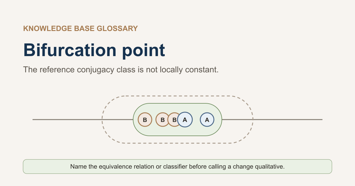
A bifurcation point is a parameter where nearby systems do not all retain the selected qualitative equivalence. The equivalence or classifier must be named. In this project’s first discrete-time interface, the primary relation is topological conjugacy by a homeomorphism of the whole state space.
Start with zero, one, and two fixed points
For each real parameter \(\mu\), consider
\[ F_\mu(x)=x+(\mu-x^2). \]The fixed-point equation is
\[ F_\mu(x)=x\iff \mu=x^2. \]It follows that negative parameters have no real fixed point, zero has the single fixed point \(x=0\), and positive parameters have the two fixed points \(x=\pm\sqrt\mu\). The calculation covers every real solution, so it establishes those counts for this family.
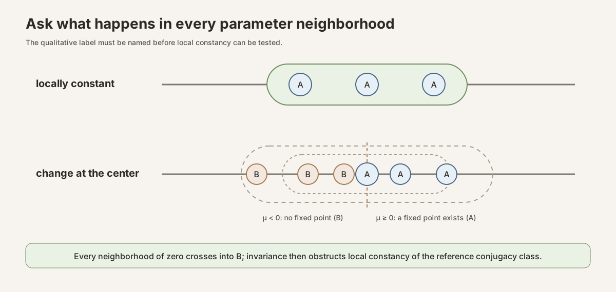
Fixed-point existence changes at \(\mu=0\): every neighborhood of zero contains negative parameters without a fixed point, while the map at zero has a fixed point. Because a topological conjugacy sends fixed points to fixed points, those nearby maps cannot all be conjugate to the map at zero.
Local constancy is a neighborhood statement
Given a classifier \(c:P\to C\), local constancy at \(\mu\) means that some neighborhood of \(\mu\) has the single value \(c(\mu)\). A change at \(\mu\) means that no such neighborhood exists.
In filter notation, the project writes
\[ \neg\bigl(\forall^\mathrm{eventually}_{\nu\to\mu}, c(\nu)=c(\mu)\bigr). \]This is equivalent to different classifier values occurring frequently near \(\mu\), meaning that every neighborhood meets the set of parameters with a different value.
An isolated parameter cannot satisfy this classifier-change definition. If \(\{\mu\}\) is open, it is itself a neighborhood on which every classifier is constant. This is why a finite regime table with the discrete topology is an illustration of cases, not by itself a real-parameter bifurcation theorem.
Parameter is not time
A family has type
\[ F:P\to(X\to X). \]The parameter \(\mu\in P\) selects a self-map \(F_\mu\). Iteration time \(n\in\mathbb N\) then selects the iterate \(F_\mu^n\). Varying \(\mu\) compares different systems. Varying \(n\) follows one orbit in a selected system.
A fixed-point branch is a function \(b:P\to X\) satisfying
\[ F_\mu(b(\mu))=b(\mu) \]on a stated parameter set. Its graph lies in parameter-state space and is not an orbit. Continuity or differentiability of the branch is extra structure, not part of the pointwise equation.
A specified-period branch satisfies \(F_\mu^n(b(\mu))=b(\mu)\). The displayed \(n\) need not be the least positive period. Fixed points satisfy the equation for every natural number.
The selected topological definition
For a parameterized family of maps on a topological space \(X\), the source defines a whole-state-space conjugacy bifurcation at \(\mu\) by
\[ \neg\bigl(\forall^\mathrm{eventually}_{\nu\to\mu}, F_\nu\text{ is globally topologically conjugate to }F_\mu\bigr). \]In the Lean declaration name, “Global” means that the homeomorphism acts on the whole state space. It does not classify the quadratic event as a global bifurcation in the standard local/global sense; the fold-type fixed-point event is local in that taxonomy. Local bifurcation theory may instead compare maps only near one fixed point, periodic orbit, or invariant set. This first definition also does not require the conjugating homeomorphisms to vary continuously with the parameter.
The source then provides a general sufficient-witness theorem. If a classifier is invariant under the relevant conjugacies and it changes at \(\mu\), then \(\mu\) satisfies the whole-state-space conjugacy bifurcation predicate.
Fixed-point existence and existence of a point with a specified period are two included classifiers. A literal fixed-point set is not used: a coordinate change can move its elements without changing the qualitative dynamics.
In Lean
def IsGlobalTopologicalBifurcationAt\n [TopologicalSpace P] [TopologicalSpace X]\n (family : ParameterizedFamily P X) (μ : P) : Prop :=\n ¬∀ᶠ ν in 𝓝 μ, AreTopologicallyConjugate (family ν) (family μ)P is the parameter type and X is the state type. Both carry topologies.
𝓝 μ is the neighborhood filter. ∀ᶠ means “eventually,” or throughout
some neighborhood. AreTopologicallyConjugate says that a homeomorphism of
the state space intertwines the two maps.Try it in the repository
Create a reader worksheet containing:
import NonlinearDynamics.Deterministic.Discrete.Bifurcation

open NonlinearDynamics.Deterministic.Discrete

#check IsGlobalTopologicalBifurcationAt
#check isGlobalTopologicalBifurcationAt_iff_frequently_not_conjugate
#check quadraticFixedPointFamily_isGlobalTopologicalBifurcationAt_zero
import loads the exact project module. open makes this milestone’s
namespace available without repeating its full prefix. The three #check
commands inspect the predicate, its neighborhood-filter form, and the worked
theorem at zero. They query already checked declarations.
This is a full project check on macOS or Linux. The pinned Mathlib environment may require substantial initial disk space and build time.
NonlinearDynamics/Deterministic/Discrete/Bifurcation.lean; the command below
checks the complete module with the repository’s pinned environment.cd formalization
lake env lean -DwarningAsError=true NonlinearDynamics/Deterministic/Discrete/Bifurcation.leanResource note: this exact file uses the repository's
pinned Lean and Mathlib dependencies. Initial project setup can require
substantial disk space and build time. For a lightweight first step on
macOS or Linux, use the page's standalone Lean-core or Std
tutorial.
The literal underlying command is:
cd formalization
lake env lean -DwarningAsError=true \
  NonlinearDynamics/Deterministic/Discrete/Bifurcation.lean
For a bounded standalone tutorial, run the finite regime worksheet, which
imports only Std:
elan run leanprover/lean4:v4.32.0 lean \
  site/content/knowledge-base/deep-dives/parameter-families-branches-and-bifurcation-in-discrete-time/finite-branch-table.lean
The worksheet checks an exhaustive finite table. It does not establish the real-parameter neighborhood theorem.
Common confusions
| Confusion | Correction |
|---|---|
| A fixed point moved, so a bifurcation occurred. | Coordinate motion alone can preserve conjugacy. |
| A branch is a trajectory. | A branch varies a parameter; a trajectory varies iteration time. |
| Two-step return means least period two. | A fixed point also returns after two steps. |
| One classifier stayed constant, so no bifurcation occurred. | A coarser classifier can miss other qualitative changes. |
| A plot found the threshold. | A plot illustrates; a complete argument or theorem establishes the stated result. |
| Nonhyperbolicity is enough for a generic normal form. | Generic classification needs regularity and nondegeneracy hypotheses. |
What this chapter does not claim
This chapter does not supply local phase-space equivalence, smooth parameter dependence, derivative or multiplier tests, hyperbolicity, genericity, transversality, codimension, fold or flip normal-form theorems, Neimark-Sacker bifurcation, stability exchange, least-period branches, continuation algorithms, numerical detection, structural stability in a topology on maps, chaos, stochastic bifurcation, or ODE bifurcation theory.
Continue with Parameter Families, Branches, and Bifurcation in Discrete Time for the worked example and standalone worksheet, or the Development Notebook for the declaration map and design decision.
References
- John Guckenheimer, “Bifurcation,” Scholarpedia 2(6):1517 (2007), DOI 10.4249/scholarpedia.1517.
- Yuri A. Kuznetsov, Elements of Applied Bifurcation Theory, 3rd ed., Applied Mathematical Sciences 112, Springer (2004), Chapters 2 and 4, DOI 10.1007/978-1-4757-3978-7.
- Yuri A. Kuznetsov, “Saddle-node bifurcation for maps,” Scholarpedia 3(4):4399 (2008), DOI 10.4249/scholarpedia.4399.
- Yuri A. Kuznetsov and Hil G. E. Meijer, Numerical Bifurcation Analysis of Maps: From Theory to Software, Cambridge University Press (2019), Chapter 2, DOI 10.1017/9781108585804.