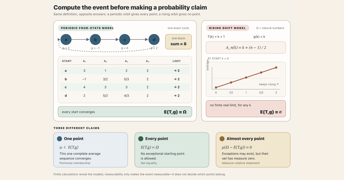
Start with four states in a repeating orbit:
\[ a\xrightarrow{T}b\xrightarrow{T}c\xrightarrow{T}d\xrightarrow{T}a. \]An observable \(g\) assigns a real reading to each state:
\[ g(a)=3,\qquad g(b)=-1,\qquad g(c)=4,\qquad g(d)=2. \]For a starting state \(x\), the Birkhoff average \(A_n^g(x)\) is the mean of the first \(n\) readings along its orbit. Here are the first four positive-time averages from every possible start:
| start \(x\) | first four readings | \(A_1,A_2,A_3,A_4\) | eventual limit |
|---|---|---|---|
| \(a\) | \(3,-1,4,2\) | \(3,1,2,2\) | \(2\) |
| \(b\) | \(-1,4,2,3\) | \(-1,\frac32,\frac53,2\) | \(2\) |
| \(c\) | \(4,2,3,-1\) | \(4,3,3,2\) | \(2\) |
| \(d\) | \(2,3,-1,4\) | \(2,\frac52,\frac43,2\) | \(2\) |
Why does looking at four terms settle an infinite-limit question here? Every complete block of four readings is a cyclic rearrangement of the same list, so every such block sums to
\[ 3+(-1)+4+2=8. \]Write a positive horizon as \(n=4q+r\), where \(0\le r\lt4\). For each start \(x\), its sum has the form
\[ S_n^g(x)=8q+R_r(x), \qquad A_n^g(x)-2=\frac{R_r(x)-2r}{4q+r}. \]Only four possible remainders \(R_r(x)\) occur, so the numerator in the last fraction stays bounded while the denominator grows. Thus every row converges to \(8/4=2\).
The Birkhoff convergence event is the set of starts whose full average sequence converges to some finite real number. We have computed the entire set in this example:
\[ E(T,g)=\{a,b,c,d\}=\Omega. \]If we put the uniform probability measure on the four states, each point has mass \(1/4\), so \(\mu(E(T,g))=1\). But the set equality \(E(T,g)=\Omega\) was proved before introducing a measure; it is a stronger, every-point statement.
Now deliberately change the model. Let \(\Omega=\mathbb N\), let \(T(k)=k+1\), and read \(g(k)=k\). Starting at \(k\),
\[ A_n^g(k) =\frac{k+(k+1)+\cdots+(k+n-1)}{n} =k+\frac{n-1}{2} \qquad(n\gt0). \]These averages rise without bound, so they do not converge to a finite real number. No starting point belongs:
\[ E(T,g)=\varnothing. \]The two models show why the word event must not be read as “something that happens.” It means a subset of the state space. Depending on \(T\) and \(g\), that subset can be all points, no points, or something in between.
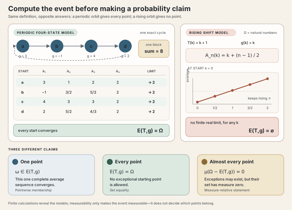
Pointwise, everywhere, and almost everywhere
These three sentences are not interchangeable:
| Scope | Paper statement | Meaning |
|---|---|---|
| one starting point | \(\omega\in E(T,g)\) | this one average sequence converges |
| every starting point | \(E(T,g)=\Omega\) | every average sequence converges |
| almost every starting point | \(\forall^\mu\omega,\ \omega\in E(T,g)\) | the set of failures is a null set |
An almost-everywhere statement can allow exceptional points. For example, a single point has probability zero under many continuous probability distributions , so a theorem may hold almost everywhere while failing at that point. On our uniform four-point space, however, every point has positive mass \(1/4\); the only null set is the empty set, and “almost every point” really does mean every point.
The twenty-second random-matrix-theory milestone (RMT-22) isolates the event,
proves its measurability under ordinary measurability assumptions, proves that
it is unchanged when the orbit is shifted by one step, and derives conditional
null-or-conull and probability-zero-or-one results. Those structural results
do not choose whether the event is empty or full. A later analytic theorem
must prove membership. This repository’s later
PointwiseBirkhoff module supplies almost-everywhere membership
under finite-measure, measure-preservation, and integrability assumptions.
The underlying finite sums are introduced in the Birkhoff sum entry. The present term adds one existential limit statement around those finite objects.
Exact definition
Let:
- \(\Omega\) be a state space;
- \(T:\Omega\to\Omega\) be a discrete-time map;
- \(g:\Omega\to\mathbb R\) be a real observable;
- \(n\in\mathbb N\) be a finite horizon; and
- \(\omega\in\Omega\) be a starting point.
The finite Birkhoff average is
\[ A_n^g(\omega) {} = \frac{1}{n}\sum_{\substack{j\in\mathbb N\\j\lt n}} g\bigl(T^j\omega\bigr). \]Mathlib totalizes division, so \(A_0^g(\omega)=0\). This time-zero value is a convenient finite convention. It does not constrain any separately defined process value \(X_0(\omega)\).
The convergence event is
\[ E(T,g) {} = \left\{\omega\in\Omega: \exists c\in\mathbb R,\ A_n^g(\omega)\longrightarrow c\right\}. \]The Lean definition is deliberately literal:
def birkhoffConvergenceSet (T : Ω → Ω) (g : Ω → ℝ) : Set Ω :=
  {ω | ∃ c : ℝ,
    Tendsto (fun n ↦ birkhoffAverage ℝ T g n ω) atTop (nhds c)}
The simp theorem mem_birkhoffConvergenceSet_iff exposes this
definition at a point. It is useful because later proofs can rewrite set
membership into an explicit limit witness without unfolding unrelated
implementation details.
In Lean: one starting point belongs
ω ∈ birkhoffConvergenceSet T g ↔ ∃ c : ℝ, Tendsto (fun n ↦ birkhoffAverage ℝ T g n ω) atTop (nhds c)ω ∈ …is ordinary membership of one point in one set.∃ c : ℝasks for a finite real witness. A sequence escaping to \(+\infty\) does not satisfy this existential statement.fun n ↦ …builds the sequence whose \(n\)-th term is the finite Birkhoff average atω.atTopmeans that natural-number horizons become arbitrarily large. It is Lean’s filter-level version of \(n\to\infty\).nhds cis the collection of neighborhoods of \(c\).Tendsto sequence atTop (nhds c)says that the sequence eventually enters every neighborhood of \(c\).mem_birkhoffConvergenceSet_iffis the exact theorem name that exposes this statement; its proof isrflbecause the set was defined by this predicate.
In Lean: almost every starting point belongs
∀ᵐ ω ∂μ, ω ∈ birkhoffConvergenceSet T g∀ᵐis Lean’s “for almost every” binder; it is not the ordinary universal quantifier∀.∂μnames the measure with respect to which exceptional sets are negligible.- The body after the comma is still pointwise membership. The binder changes how many exceptions are permitted.
- This line is a proposition to prove, not a consequence of the definition.
In the later
PointwiseBirkhoffmodule, the exact theoremae_mem_birkhoffConvergenceSet_of_integrableproves it from a finite measure, a measure-preserving map, and an integrable observable.
Four statements that must stay separate
The following claims answer different questions:
| Layer | Representative claim | What it controls |
|---|---|---|
| Finite | every \(A_n^g\) is measurable or integrable | one fixed horizon |
| Event | \(E(T,g)\) is measurable or null measurable | whether the set is legitimate for measure theory |
| Rigidity | \(E(T,g)\) is null or conull under ergodicity | the only possible sizes if it is invariant |
| Existence | almost every point lies in \(E(T,g)\) | actual convergence |
RMT-22 proves the first three layers under their stated hypotheses. That
module does not prove the fourth; the later PointwiseBirkhoff
module does so under additional analytic hypotheses. In particular, the
RMT-22 disjunction
does not choose the second branch. The pointwise Birkhoff ergodic theorem is the kind of analytic result that supplies almost-everywhere membership under additional hypotheses.
Why the event is measurable
In either cold-open model, give the countable state space its full power-set \(\sigma\)-algebra. Every subset is then measurable, so \(\Omega\) and \(\varnothing\) are measurable by inspection. A general state space can have a smaller \(\sigma\)-algebra, however, and the conclusion then needs an argument.
Suppose \(T\) and \(g\) are ordinarily measurable. Every iterate \(T^j\) is measurable, so every finite composition \(g\circ T^j\) is measurable. A finite sum of those functions is measurable, and multiplication by the constant \(n^{-1}\) preserves measurability. Therefore each map
\[ \omega\longmapsto A_n^g(\omega) \]is measurable.
For a sequence of real-valued measurable functions, the set of points where
the sequence converges to some real limit is measurable. RMT-22 applies
Mathlib’s
MeasureTheory.measurableSet_exists_tendsto
to obtain
measurableSet_birkhoffConvergenceSet. No probability,
integrability, preservation, or ergodicity assumption is needed for this
ordinary-measurability route.
measurableSet_birkhoffConvergenceSet hT hghT : Measurable Tis the proof that inverse images under the dynamics respect the chosen \(\sigma\)-algebra.hg : Measurable gis the corresponding proof for the observable.- The result has type
MeasurableSet (birkhoffConvergenceSet T g). - No
MeasurePreserving,Integrable, orErgodictoken appears because none is needed for this theorem. - Measurable means the set can be assigned a measure. It says nothing about whether that measure is zero, one, or somewhere between.
Why integrability does not imply ordinary measurability
In Mathlib, Integrable g μ contains almost-everywhere strong
measurability, not an assertion that the supplied representative \(g\) is
ordinarily measurable at every point. Replacing that premise by
Measurable g would silently strengthen the theorem.
RMT-22 instead starts from AEMeasurable g μ. Mathlib’s
almost-everywhere measurable representative API
provides an ordinarily measurable representative hg.mk g such that
If \(T\) is quasi-measure-preserving, an almost-everywhere equality remains available along every finite orbit iterate. The finite Birkhoff averages of the two representatives are consequently equal almost everywhere at every horizon. Their convergence events are therefore equal almost everywhere. This proves that the original event is null measurable: it agrees almost everywhere with a measurable set.
The public interface exposes three assumption levels:
…_of_aemeasurableis the primary representative theorem;…_of_aestronglyMeasurableis an ergonomic corollary; and…_of_integrableuses only the measurability field of integrability.
Quasi-measure preservation matters. Without it, a null exceptional set for \(g=h\) need not remain null after taking preimages along the orbit.
Exact preimage invariance
The finite averages at \(\omega\) and \(T\omega\) differ only by a finite prefix. For positive indices, RMT-22 proves both algebraic identities
\[ \begin{aligned} A_{n+1}^g(T\omega) &=\frac{n+2}{n+1}A_{n+2}^g(\omega) -\frac{g(\omega)}{n+1},\\ A_{n+2}^g(\omega) &=\frac{g(\omega)}{n+2} +\frac{n+1}{n+2}A_{n+1}^g(T\omega). \end{aligned} \]The rational coefficients tend to one and the one-point correction tends to zero. Hence convergence at \(\omega\) to \(c\) is equivalent to convergence at \(T\omega\) to the same \(c\). No measurability, boundedness, preservation, injectivity, surjectivity, or invertibility premise is used.
Existentially quantifying the common limit gives the exact set equation
\[ T^{-1}\bigl(E(T,g)\bigr)=E(T,g). \]This is preimage invariance. RMT-22 makes no image-invariance claim. When \(T\) is not surjective, equality with \(T(E(T,g))\) is a different statement and does not follow from this proof.
Ergodic rigidity remains conditional
For an ordinarily measurable event, exact preimage invariance and
PreErgodic T μ already give the almost-everywhere empty-or-full
dichotomy. The full measure-preservation component of Ergodic is
not consumed by that route.
For a merely null-measurable event, the corresponding
Mathlib theorem uses
QuasiErgodic T μ. RMT-22 therefore keeps that receiver on its
generic representative-safe theorem. An ordinary ergodic hypothesis can be
passed through hT.quasiErgodic when desired.
On a probability space, the two branches become the numerical zero-one law
\[ \mu(E(T,g))=0 \qquad\text{or}\qquad \mu(E(T,g))=1. \]Again, this is a dichotomy, not an existence theorem. On the zero measure, the almost-everywhere empty and almost-everywhere full descriptions are both vacuous because every set agrees almost everywhere with every other set.
Boundary models and edge cases
Zero and constant observables
If \(g=0\), every finite average is zero, so \(E(T,g)=\Omega\) for every map \(T\). If \(g\equiv c\), the time-zero average is zero but every positive-time average is \(c\). Removing the first term of a sequence does not change its limit, so the convergence event is still all of \(\Omega\).
Identity dynamics
If \(T\) is the identity, the orbit never leaves \(\omega\). For every positive \(n\),
\[ A_n^g(\omega)=g(\omega). \]Thus every point belongs to the event, even if \(g\) is not measurable. This is a pointwise algebraic fact, not a measure-theoretic one.
A genuinely divergent orbit
Let the state space be the natural numbers, let \(T(k)=k+1\), let \(g(k)=k\), and start at \(k\). For every positive \(n\),
\[ A_n^g(k)=k+\frac{n-1}{2}. \]The sequence tends to positive infinity, not to a finite real. Hence no natural-number start belongs and \(E(T,g)=\varnothing\). The compiled RMT-22 boundary probe checks the start at zero, while the displayed closed formula settles every \(k\).
Time zero, empty spaces, and the zero measure
- Mathlib defines \(A_0^g(\omega)=0\). Event membership still depends on the tail as \(n\to\infty\); one initial value cannot create or destroy a limit.
- If \(\Omega\) is empty, then \(E(T,g)=\varnothing=\Omega\). The phrases “empty event” and “full event” coincide because there are no points.
- Under the zero measure, every exceptional set is null. Consequently an almost-everywhere membership statement can be true even when there is no pointwise member. Never extract a concrete witness from an a.e. theorem without an additional nonvacuity argument.
A tiny standalone Lean worksheet a human can type
Standalone tutorial. This worksheet computes exact finite sums for the two cold-open models. It does not import Mathlib, define filters, or prove that an infinite sequence converges.
Save it as BirkhoffConvergenceTutorial.lean:
import Std

inductive OrbitState where
  | a | b | c | d
deriving Repr, DecidableEq

def step : OrbitState → OrbitState
  | .a => .b
  | .b => .c
  | .c => .d
  | .d => .a

def reading : OrbitState → Int
  | .a => 3
  | .b => -1
  | .c => 4
  | .d => 2

def iterate : Nat → OrbitState → OrbitState
  | 0, x => x
  | n + 1, x => iterate n (step x)

def orbitSum : Nat → OrbitState → Int
  | 0, _ => 0
  | n + 1, x => orbitSum n x + reading (iterate n x)

-- The pair (sum, horizon) represents the exact average sum / horizon.
def averageFraction (n : Nat) (x : OrbitState) : Int × Nat :=
  (orbitSum n x, n)

#eval [averageFraction 1 .a, averageFraction 2 .a,
  averageFraction 3 .a, averageFraction 4 .a]
#eval [averageFraction 4 .a, averageFraction 4 .b,
  averageFraction 4 .c, averageFraction 4 .d]

example : orbitSum 4 .a = 8 := by decide
example : orbitSum 4 .b = 8 := by decide
example : orbitSum 4 .c = 8 := by decide
example : orbitSum 4 .d = 8 := by decide
example : orbitSum 8 .a = 16 := by decide
example : orbitSum 8 .d = 16 := by decide

-- 0 + 1 + ... + (n - 1), the numerator for the rising model at start 0.
def risingSum : Nat → Nat
  | 0 => 0
  | n + 1 => risingSum n + n

-- For n > 0 this is twice the average: 2 * risingSum n / n = n - 1.
def twiceRisingAverage (n : Nat) : Nat :=
  if n = 0 then 0 else (2 * risingSum n) / n

#eval [risingSum 1, risingSum 2, risingSum 3, risingSum 4, risingSum 5]
#eval [twiceRisingAverage 1, twiceRisingAverage 2,
  twiceRisingAverage 3, twiceRisingAverage 4, twiceRisingAverage 5]

example : risingSum 5 = 10 := by decide
example : twiceRisingAverage 5 = 4 := by decide
From the directory containing the file, type:
source "$HOME/.elan/env"
elan run leanprover/lean4:v4.32.0 lean BirkhoffConvergenceTutorial.lean
The first output represents \(3/1,2/2,6/3,8/4\), namely \(3,1,2,2\). The four horizon-\(4\) fractions all have numerator \(8\) and denominator \(4\). The rising-model sums are \(0,1,3,6,10\), and twice its first five positive-time averages are \(0,1,2,3,4\). These finite checks expose the pattern; the bounded-remainder and closed-form arguments above are what justify the infinite conclusions.
This command is appropriate on an ordinary Mac or Linux machine: it imports
only Std and compiles one tiny file. It is intentionally separate
from the project and Mathlib checks below. This exact worksheet was executed
successfully with the pinned Lean 4.32.0 compiler.
Try the exact project declarations
Full project check. This uses the repository’s pinned Lean and Mathlib dependencies and may require substantial disk space and memory. Create a temporary project worksheet containing:
import NonlinearDynamics.Random.RandomCocycles.BirkhoffConvergence

open NonlinearDynamics.Random.RandomCocycles

#check birkhoffConvergenceSet
#check mem_birkhoffConvergenceSet_iff
#check measurableSet_birkhoffConvergenceSet
#check birkhoffConvergenceSet_ae_eq_of_ae_eq
#check nullMeasurableSet_birkhoffConvergenceSet_of_integrable
#check tendsto_birkhoffAverage_apply_base_iff
#check preimage_birkhoffConvergenceSet
#check birkhoffConvergenceSet_ae_empty_or_univ_of_measurableSet
#check measure_birkhoffConvergenceSet_eq_zero_or_one_of_integrable
Each #check asks the pinned elaborator for a declaration’s exact
type. The full-project command below compiles the authoritative RMT-22 module. It
uses the repository’s pinned Lean and Mathlib dependencies and may require
substantial disk space and memory.
cd formalization
lake env lean -DwarningAsError=true NonlinearDynamics/Random/RandomCocycles/BirkhoffConvergence.lean
Resource note: this exact file uses the repository's
pinned Lean and Mathlib dependencies. Initial project setup can require
substantial disk space and build time. For a lightweight first step on
macOS or Linux, use the page's standalone Lean-core or Std
tutorial.
Resource label: later pinned project theorem. To see the distinction between defining the event and proving almost-everywhere membership, query the later module:
import NonlinearDynamics.Random.RandomCocycles.PointwiseBirkhoff

open NonlinearDynamics.Random.RandomCocycles

#check ae_mem_birkhoffConvergenceSet_of_integrable
That theorem assumes a finite measure, measure-preserving dynamics, and an integrable real observable. Its conclusion is the exact almost-everywhere Lean sentence displayed above. It does not identify the value of the limit. The full-project command compiles the later authoritative module with the repository’s pinned dependencies.
cd formalization
lake env lean -DwarningAsError=true NonlinearDynamics/Random/RandomCocycles/PointwiseBirkhoff.lean
Resource note: this exact file uses the repository's
pinned Lean and Mathlib dependencies. Initial project setup can require
substantial disk space and build time. For a lightweight first step on
macOS or Linux, use the page's standalone Lean-core or Std
tutorial.
Candidate and matrix-cocycle views
For an integrable shifted-subadditive-process candidate \(X\), RMT-22 names
\[ E_1(T,X)=E(T,X_1). \]Only the one-step observable appears. The value \(X_0\) can be nonzero. The compiled boundary model constructs a valid candidate over the zero measure with \(X_0=1\) and \(X_n=0\) for positive \(n\); its one-step convergence event is still the whole space.
For a discrete matrix cocycle \(C\), the named event uses the measurable one-step log-positive norm observable
\[ \omega\longmapsto \log^+\lVert C(1,\omega)\rVert_\infty. \]Ordinary measurability comes from the cocycle itself. The event-measurability,
exact-invariance, and pre-ergodic rigidity wrappers require no
HasIntegrableGeneratorLogPlus premise and no nonempty matrix-index
premise. The empty matrix index is an explicit compiled probe.
The 37-declaration interface at a glance
The frozen RMT-22 source exposes exactly thirty-seven public declarations:
| Family | Count | Responsibility |
|---|---|---|
| Finite sum and average | 4 | measurability and integrability |
| Event and representatives | 7 | definition, membership, measurability, and representative transport |
| Shift and exact invariance | 6 | two identities, two limit directions, an equivalence, and a preimage equation |
| Generic rigidity and zero-one laws | 10 | measurable and null-measurable paths plus three representative corollaries each |
| Candidate specialization | 5 | one-step event and conditional wrappers |
| Matrix-cocycle specialization | 5 | generator event and conditional wrappers without generator integrability |
The long Deep Dive lists all declaration names and reconstructs their proof dependencies.
What the term does not claim
A Birkhoff convergence event, even when measurable and invariant, does not by itself establish:
- membership of any specified point;
- nonemptiness, positive measure, or full measure;
- almost-everywhere convergence;
- identification of a limit with a space average;
- convergence in integrable norm, probability, or distribution;
- a maximal ergodic inequality;
- the pointwise Birkhoff ergodic theorem;
- Kingman’s subadditive ergodic theorem;
- mixing, independence, or decay of correlations;
- a Lyapunov exponent; or
- an Oseledets filtration or splitting.
Where to continue
The almost everywhere entry explains the equality notion used for representatives and events. The ergodic probability base entry separates probability normalization, preservation, ergodicity, and integrability.
Birkhoff Convergence Events Before the Pointwise Ergodic Theorem develops the complete textbook route, solved exercises, and declaration map.
The finite maximal ergodic inequality entry develops the next analytic ingredient: a strict finite running-maximum event whose integral is nonnegative, followed by a horizon-uniform weak threshold estimate. It still does not place almost every point in the convergence event.
Finite Ordered Interval Packing for Nonpositive Subadditive Processes is the finite combinatorial predecessor. RMT-22 supplies an event interface, but it still does not supply the density or convergence theorem needed to complete the later Kingman argument.
References
All Mathlib links below refer to the v4.32.0 API used by this project. The
pinned local checkout at commit
81a5d257c8e410db227a6665ed08f64fea08e997 is the exact source
authority.
Mathlib contributors. Birkhoff averages, with the pinned definition and time-zero theorem. These sources define the totalized finite average reused by RMT-22.
Mathlib contributors. Birkhoff averages under quasi-measure-preserving maps, with the pinned representative-transport theorem. This is the finite almost-everywhere transport used before event congruence.
Mathlib contributors.
Almost-everywhere measurable representatives,
with the
pinned AEMeasurable.mk, measurable_mk, and
ae_eq_mk API.
This is the ordinary representative used by the primary
AEMeasurable route.
Mathlib contributors. Polish-space measure constructions, with the pinned convergence-set theorem. The theorem proves measurability of the points where a measurable sequence has some limit in a completely metrizable second-countable target such as the reals.
Mathlib contributors. Ergodic maps and measures, with the pinned pre-ergodic and quasi-ergodic rigidity theorems. The same source contains the null-measurable quasi-ergodic path used by the representative-safe interface.
George D. Birkhoff. Proof of the Ergodic Theorem, Proceedings of the National Academy of Sciences 17(12), 656-660, 1931. The archival record gives DOI 10.1073/pnas.17.2.656. This primary source is the historical pointwise convergence theorem. RMT-22 formalizes only the finite and conditional event infrastructure before such a theorem.
The exact upstream revision is commit
81a5d257,
the v4.32.0 revision pinned by formalization/lake-manifest.json.