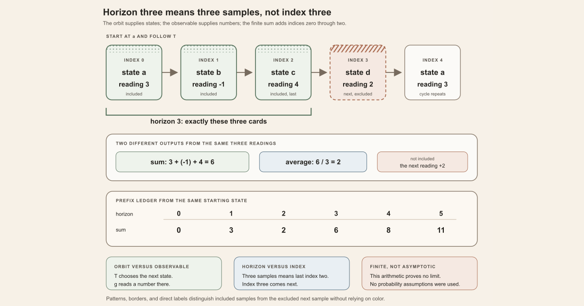
Start with four states arranged in a cycle:
\[ a\xrightarrow{T}b\xrightarrow{T}c\xrightarrow{T}d\xrightarrow{T}a. \]The map \(T\) tells us where to move. A separate function \(g\), called an observable, tells us what number to read at each state:
\[ g(a)=3,\qquad g(b)=-1,\qquad g(c)=4,\qquad g(d)=2. \]Beginning at \(a\), the orbit states are
\[ a,\ b,\ c,\ d,\ a,\ldots \]and the observed readings are
\[ 3,\ -1,\ 4,\ 2,\ 3,\ldots . \]A Birkhoff sum of horizon \(n\) adds the first \(n\) readings. The first six prefix sums are therefore:
| horizon \(n\) | sampled indices | readings added | Birkhoff sum |
|---|---|---|---|
| \(0\) | none | empty sum | \(0\) |
| \(1\) | \(0\) | \(3\) | \(3\) |
| \(2\) | \(0,1\) | \(3+(-1)\) | \(2\) |
| \(3\) | \(0,1,2\) | \(3+(-1)+4\) | \(6\) |
| \(4\) | \(0,1,2,3\) | \(3+(-1)+4+2\) | \(8\) |
| \(5\) | \(0,1,2,3,4\) | \(3+(-1)+4+2+3\) | \(11\) |
At horizon \(3\), three terms are included and the last index is \(2\). The state \(d\), at index \(3\), is the next sample and is not included. This is the off-by-one convention to remember:
\[ \text{horizon }n =\text{number of samples}, \qquad \text{last included index}=n-1 \quad(n\gt0). \]The corresponding average at horizon \(3\) is \(6/3=2\). The sum is \(6\); the average is \(2\). Dividing is a separate operation.
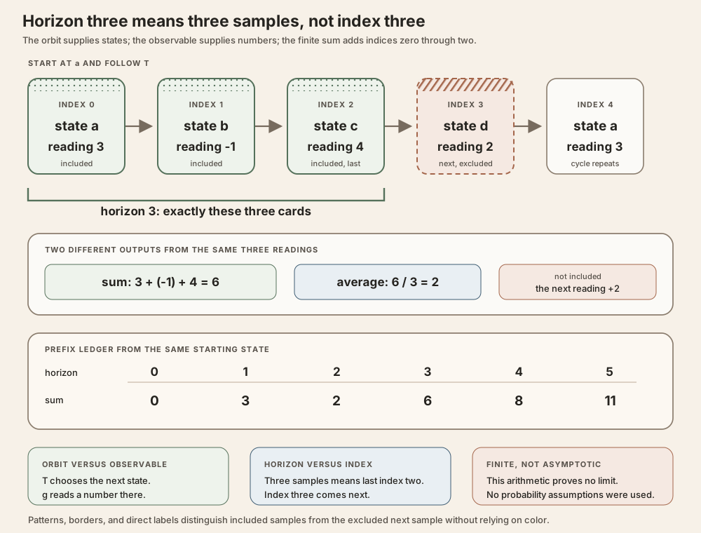
Nothing probabilistic was needed. We fixed one starting point, followed one finite orbit, evaluated one function, and added finitely many integers. A probability measure , measure preservation , integrability , and ergodicity enter only in later theorems.
For the finite-block estimates in the eighteenth Random Matrix Theory milestone (RMT-18), the same construction is reused with the powered orbit map \(T^b\) and the complete-block observable \(X_b\). That advanced use comes after the basic definition below.
The exact finite definition
Let \(\Omega\) be a state space, let \(S:\Omega\to\Omega\) be a map, let \(F:\Omega\to\mathbb R\) be an observable, let \(q\in\mathbb N\), and let \(\omega\in\Omega\). The length-\(q\) Birkhoff sum is
\[ \operatorname{BSum}(S,F,q,\omega) {} = \sum_{\substack{j\in\mathbb N\\j\lt q}} F\bigl(S^j\omega\bigr). \]Mathlib, Lean’s community mathematics library, writes this as
birkhoffSum S F q ω and implements the finite index set as
Finset.range q. Thus the first index is zero and the last index,
when \(q\) is positive, is \(q-1\). At \(q=0\), the range is empty and the
sum is zero. These are definitional finite-sum facts, not measure-theoretic
claims (pinned Mathlib source).
Four distinctions that prevent most mistakes
- Orbit versus observable. The orbit is the state sequence \(\omega,S\omega,S^2\omega,\ldots\). The observable \(F\) turns each state into an addable value. In the cold-open example, \(T(a)=b\), but \(g(a)=3\). The map returns a state; the observable returns a number.
- Horizon versus last index. Horizon \(q\) means \(q\) samples, indexed \(0\) through \(q-1\) when \(q\gt0\). Horizon \(3\) does not include index \(3\).
- Sum versus average. The Birkhoff sum is \(\sum_{j=0}^{q-1}F(S^j\omega)\). For positive \(q\), the Birkhoff average divides that sum by \(q\). They have different values and different Lean names.
- Finite arithmetic versus convergence. Computing one value at one horizon proves nothing about what happens as \(q\to\infty\). A convergence theorem needs additional analytic and dynamical hypotheses.
Mathlib totalizes the zero-horizon average as zero:
\[ \operatorname{BAvg}(S,F,0,\omega)=0. \]On paper, “sum divided by the number of samples” is undefined at zero samples. The Lean definition uses the inverse of the scalar \(0\), which is \(0\) in the relevant division semiring, so its zero case is an explicit library convention rather than ordinary division by zero.
The four inputs have distinct jobs:
| Input | Meaning in a general Birkhoff sum | RMT-18 block interpretation |
|---|---|---|
| \(S\) | orbit map | powered base map \(T^b\) |
| \(F\) | value sampled on the orbit | block observable \(X_b\) |
| \(q\) | number of samples | number of complete blocks |
| \(\omega\) | initial state | sample where the block train starts |
Confusing any two columns changes the theorem. In particular,
birkhoffSum T (X b) q ω samples the block cost after every one-step
move. RMT-18 needs birkhoffSum (T^[b]) (X b) q ω, which samples it
after every \(b\)-step move.
Powered-base sampling
Fix a block length \(b\) and set \(S=T^b\). Iterating the powered map \(j\) times advances \(bj\) one-step times:
\[ S^j\omega {} = \bigl(T^b\bigr)^j\omega {} = T^{bj}\omega. \]When \(q\) is positive, the block Birkhoff sum expands as
\[ \begin{aligned} \operatorname{BSum}(T^b,X_b,q,\omega) &= \sum_{\substack{j\in\mathbb N\\j\lt q}} X_b\bigl(T^{bj}\omega\bigr) \\ &= X_b(\omega)+X_b(T^b\omega)+\cdots +X_b\bigl(T^{b(q-1)}\omega\bigr). \end{aligned} \]This sum has \(q\) terms, not \(bq\) terms. Each term already summarizes a horizon of length \(b\). The powered map supplies the spacing between block starts.
This is the first useful mental model: a Birkhoff sum is an orbit sampler. The map determines where to sample, the observable determines what to read, and the horizon determines how many readings to add.
The recurrence laws expose both ends
Mathlib supplies two successor recurrences for the same finite sum (official recurrence documentation):
\[ \begin{aligned} \operatorname{BSum}(S,F,q+1,\omega) &= \operatorname{BSum}(S,F,q,\omega)+F(S^q\omega), \\ \operatorname{BSum}(S,F,q+1,\omega) &= F(\omega)+\operatorname{BSum}(S,F,q,S\omega). \end{aligned} \]The first equation appends the last sampled value. The second peels off the first sampled value and shifts the initial point. Neither orientation is more true. Each matches a different induction.
The addition law splits a longer sum after \(m\) samples:
\[ \operatorname{BSum}(S,F,m+n,\omega) {} = \operatorname{BSum}(S,F,m,\omega) {} + \operatorname{BSum}(S,F,n,S^m\omega). \]RMT-18 uses the successor laws to align repeated subadditivity with the powered orbit. The library identities prevent an informal index shift from quietly changing a block start.
From shifted subadditivity to complete blocks
Let \(X_n(\omega)\) be a real cost for a horizon of length \(n\). The RMT-17 process candidate stores the pointwise inequality
\[ X_{m+k}(\omega) \le X_k(T^m\omega)+X_m(\omega). \]It also stores integrability of each \(X_n\), but that analytic field is not used in the pointwise block bounds. Repeatedly apply the inequality with complete blocks of length \(b\). The complete-block terms line up at the powered-orbit points
\[ \omega,\ T^b\omega,\ T^{2b}\omega,\ldots . \]Their sum is exactly a Birkhoff sum of the observable \(X_b\) under the map \(T^b\). The Birkhoff vocabulary is useful because it packages the otherwise error-prone finite index bookkeeping into a standard object.
Terminal-remainder orientation
Write a horizon as \(bq+r\): first \(q\) complete blocks, then a remainder of length \(r\). RMT-18 proves
\[ X_{bq+r}(\omega) \le \operatorname{BSum}(T^b,X_b,q,\omega) {} + X_r\bigl((T^b)^q\omega\bigr). \]The complete blocks begin at one-step orbit times \(0,b,2b,\ldots,(q-1)b\). The terminal remainder begins at time \(bq\). No assumption about \(X_0\) is needed. When \(q=0\), the Birkhoff sum is empty and the statement reduces to \(X_r(\omega)\le X_r(\omega)\).
Substituting Euclidean division gives a theorem for every natural horizon:
\[ \begin{aligned} X_n(\omega) \le{}& \operatorname{BSum}\left(T^b,X_b,\left\lfloor\frac nb\right\rfloor,\omega\right) \\ &+X_{n\bmod b}\left((T^b)^{\lfloor n/b\rfloor}\omega\right). \end{aligned} \]For positive \(b\), the remainder satisfies \(n\bmod b\lt b\). That strict remainder bound needs \(0\lt b\); the inequality itself does not.
Remainder-first orientation
The same horizon can be written as \(r+bq\): first the short remainder, then the complete blocks. RMT-18 proves the complementary estimate
\[ X_{r+bq}(\omega) \le X_r(\omega) {} + \operatorname{BSum}(T^b,X_b,q,T^r\omega). \]Now the remainder stays at the original sample. The block train begins after that remainder, so its sampled block starts occur at one-step orbit times \(r,r+b,r+2b,\ldots,r+(q-1)b\). This theorem also needs no assumption about \(X_0\). At \(q=0\), it reduces to the same reflexive inequality as the terminal-remainder form.
The quotient-and-remainder version is
\[ \begin{aligned} X_n(\omega) \le{}& X_{n\bmod b}(\omega) \\ &+\operatorname{BSum}\left( T^b,X_b,\left\lfloor\frac nb\right\rfloor, T^{n\bmod b}\omega\right). \end{aligned} \]This orientation is often convenient when the remainder cost has a separate finite-horizon bound at the original sample. The terminal orientation is often convenient when an induction naturally appends the short tail. RMT-18 records both instead of forcing every later proof to reverse the decomposition by hand.
Worked example: seventeen steps in blocks of five
Take \(n=17\) and \(b=5\). Natural-number division gives
\[ 17=5\cdot3+2, \qquad 17/5=3, \qquad 17\bmod5=2. \]The terminal-remainder form reads
\[ \begin{aligned} X_{17}(\omega) \le{}& X_5(\omega)+X_5(T^5\omega)+X_5(T^{10}\omega) \\ &+X_2(T^{15}\omega). \end{aligned} \]There are three complete five-step blocks beginning at times zero, five, and ten. The two-step remainder begins at time fifteen.
The remainder-first form reads
\[ \begin{aligned} X_{17}(\omega) \le{}& X_2(\omega)+X_5(T^2\omega)+X_5(T^7\omega) \\ &+X_5(T^{12}\omega). \end{aligned} \]Here the two-step remainder comes first. The three complete blocks then begin at times two, seven, and twelve. Both right sides cover a seventeen-step horizon, but they evaluate the cost functions at different orbit points. One must not replace one by the other without the corresponding subadditive argument.
The zero-count boundary is exact
Shifted subadditivity at \(m=k=0\) yields
\[ X_0(\omega) \le X_0(\omega)+X_0(\omega), \]so \(X_0(\omega)\ge0\). It does not force \(X_0=0\). A constant-one process, for example, satisfies the shifted subadditive inequality and has \(X_0=1\).
For a positive number of exact blocks, RMT-18 proves
\[ X_{bq}(\omega) \le \operatorname{BSum}(T^b,X_b,q,\omega) \qquad(q\ne0) \]without a time-zero normalization. The induction has at least one block to pay for.
A theorem quantified uniformly over all block counts includes \(q=0\). At that boundary it asks for
\[ X_0(\omega)\le0. \]Combined with the forced nonnegativity, this is equivalent to \(X_0=0\). That is the only reason the uniform exact-block theorem assumes exact time-zero vanishing.
The zero-block distinction is recorded explicitly in the following table:
| Finite statement | Needs \(X_0=0\)? | What happens at zero blocks? |
|---|---|---|
| complete blocks plus terminal remainder | no | reflexive remainder bound |
| remainder plus complete blocks | no | reflexive remainder bound |
| exact blocks with \(q\ne0\) | no | zero count excluded |
| exact blocks for every \(q\) | yes | requires \(X_0\le0\) |
The remainder-first estimate does not need \(X_0=0\). Adding that assumption there would hide the actual strength of the finite algebra.
Block length zero is defined, but degenerate
Natural-number division in Lean is total. At \(b=0\), one has \(n/0=0\) and \(n\bmod0=n\). Each quotient-and-remainder block estimate therefore becomes a reflexive bound:
\[ X_n(\omega) \le 0+X_n(\omega) \]or the same two terms in the opposite order. The theorem remains valid, but there are no complete positive-length blocks to interpret. A later argument that needs the useful fact \(n\bmod b\lt b\) must add \(0\lt b\) explicitly.
Total definitions are valuable in Lean because they avoid artificial partial functions. They do not absolve the prose from explaining when a boundary case has become tautological.
Pointwise algebra does not need integrability
The two block inequalities compare real numbers at a fixed sample \(\omega\). Their proofs use shifted subadditivity, natural-number arithmetic, iterate identities, and finite-sum recurrences. They do not integrate anything. Consequently they need neither:
Integrable (X b) μ;- measure preservation;
- probability normalization; nor
- ergodicity.
The cocycle specializations preserve this narrow assumption boundary.
logPlusNormObservable_nat_mul_le_birkhoffSum and
logPlusNormObservable_le_mod_add_blockBirkhoffSum use the
log-positive norm process’s checked subadditivity. The exact-block theorem uses
the checked time-zero identity only to include the zero block count; the
remainder-first theorem needs no such normalization. Neither theorem uses
the one-step integrability hypothesis. Both remain valid when the finite
matrix index type is empty.
Finite-sum integrability needs only the block map
Integrability enters when the finite Birkhoff sum itself must be integrable. Suppose every \(X_n\) is integrable and the powered map \(S=T^b\) preserves \(\mu\). Each summand
\[ \omega\longmapsto X_b(S^j\omega) \]is integrable because \(S^j\) preserves the measure. A finite sum of
integrable real functions is integrable. This is exactly the architecture of
integrable_birkhoffSum_blocks: it uses Mathlib’s preservation of
iterates and its transport of integrability through a measure-preserving map
(measure-preserving iterates,
integrability transport).
The minimal hypothesis is
hTb : MeasurePreserving (T^[b]) μ μ
It is stronger than measurability and weaker than assuming a whole
probability-ergodic system. The theorem does not require that \(T\) itself
preserve \(\mu\), provided the particular block map \(T^b\) does. In the matrix
cocycle specialization, the cocycle already stores preservation of \(T\), so
Mathlib’s MeasurePreserving.iterate supplies preservation of
\(T^b\).
This analytic conclusion is still finite-time. It certifies one finite sum as an \(L^1\) function, meaning that its absolute value has finite integral. It does not state that normalized sums converge.
The two-cycle trap: an ergodic map can have a nonergodic power
Let \(\Omega=\{0,1\}\) with equal probabilities and let \(T\) exchange the two points. The map \(T\) is ergodic: the only strictly invariant subsets are empty and full. But \(T^2\) is the identity. Every subset is invariant under the identity, so \(T^2\) is not ergodic.
This example blocks a common shortcut. From Ergodic T μ, one
cannot generally infer Ergodic (T^[b]) μ. Lalley’s proof notes for
Kingman’s theorem call out exactly this powered-map difficulty when explaining
why a naive blockwise application of Birkhoff’s theorem is insufficient
(Lalley, Kingman notes).
RMT-18 never needs the invalid shortcut. Its pointwise bounds need no ergodicity. Its finite-sum integrability theorem needs only measure preservation of the powered map, and preservation does pass to iterates. Ergodicity and measure preservation must not be conflated.
A finite Birkhoff sum is not a Birkhoff theorem
The word Birkhoff names both a finite orbit-sum construction and famous asymptotic theorems. Importing the construction does not import their conclusions. RMT-18 proves no statement about
\[ \lim_{q\to\infty} \frac1q\operatorname{BSum}(T^b,X_b,q,\omega). \]It also proves no limit for \(X_n(\omega)/n\). Kingman’s subadditive ergodic theorem is designed to turn a measure-preserving integrable subadditive process into an almost-sure normalized limit, meaning a limit outside a set of probability zero, under additional hypotheses (Kingman, 1968). Lalley’s short proof notes show how finite block estimates participate in that much longer argument, including the need to handle the nonergodicity of powers rather than assume it away (Lalley). Their page 2 phase display is not adopted literally here: its right side counts one more complete block than its printed left-side horizon. The phase averaging entry states the corrected finite horizon and explains why that indexing repair does not change the asymptotic theorem.
Accordingly, the RMT-18 Birkhoff-sum layer establishes none of the following:
- pointwise or almost-everywhere convergence of normalized process values;
- a Birkhoff pointwise ergodic theorem;
- Kingman’s subadditive ergodic theorem;
- equality of a samplewise limit with an integrated Fekete rate;
- convergence in \(L^1\), probability, or distribution;
- independence, mixing, or decay of correlations;
- a Lyapunov exponent or Oseledets splitting; or
- ergodicity of every powered base map.
The role of this layer is narrower and indispensable: it freezes the finite indexing and assumption boundaries that any later asymptotic proof must use correctly.
In Lean: the sum in three languages
birkhoffSum S F q ωSis the self-map that generates the orbit.Fis the observable being sampled. Its output lives in an additive commutative monoid, so the values can be added and there is a zero.q : ℕis the number of samples, not the last sample index.ωis the initial state.birkhoffSumis unqualified because Mathlib defines it in the root namespace.
This is Mathlib’s exact pinned definition:
def birkhoffSum (f : α → α) (g : α → M) (n : ℕ) (x : α) : M :=
  ∑ k ∈ range n, g (f^[k] x)
Here range n is the finite set of natural numbers strictly below
n. The notation f^[k] means the \(k\)-fold iterate,
and ∑ is a finite sum.
In Lean: sum and average are different definitions
birkhoffAverage ℝ T g n ωbirkhoffAveragecallsbirkhoffSumand scales it by the inverse of the scalar cast ofn.- The explicit
ℝtells Lean to perform the scaling with real numbers. - At positive
n, this is ordinary division by the number of samples. Atn = 0, Mathlib’s total definition returns zero. - No arrow toward infinity appears in either definition. A term such as
Tendstobelongs to a separate convergence statement.
The exact pinned average definition is:
def birkhoffAverage (f : α → α) (g : α → M) (n : ℕ) (x : α) : M :=
  (n : R)⁻¹ • birkhoffSum f g n x
A tiny standalone Lean worksheet a human can type
Standalone tutorial. This file recreates only the four-state arithmetic. It does not import Mathlib, define Mathlib’s generic Birkhoff sum, or prove a convergence theorem.
Save it as BirkhoffSumTutorial.lean:
import Std

inductive OrbitState where
  | a | b | c | d
deriving Repr, DecidableEq

def step : OrbitState → OrbitState
  | .a => .b
  | .b => .c
  | .c => .d
  | .d => .a

def reading : OrbitState → Int
  | .a => 3
  | .b => -1
  | .c => 4
  | .d => 2

def iterate (T : OrbitState → OrbitState) : Nat → OrbitState → OrbitState
  | 0, x => x
  | n + 1, x => iterate T n (T x)

def orbitSum (T : OrbitState → OrbitState) (g : OrbitState → Int) :
    Nat → OrbitState → Int
  | 0, _ => 0
  | n + 1, x => orbitSum T g n x + g (iterate T n x)

def lastIncludedIndex : Nat → Option Nat
  | 0 => none
  | n + 1 => some n

#eval orbitSum step reading 0 .a
#eval orbitSum step reading 1 .a
#eval orbitSum step reading 2 .a
#eval orbitSum step reading 3 .a
#eval orbitSum step reading 4 .a
#eval orbitSum step reading 5 .a
#eval lastIncludedIndex 0
#eval lastIncludedIndex 3

example : orbitSum step reading 3 .a = 6 := by decide
example : orbitSum step reading 4 .a = 8 := by decide
example : lastIncludedIndex 3 = some 2 := by decide
From the directory containing the file, type:
source "$HOME/.elan/env"
elan run leanprover/lean4:v4.32.0 lean BirkhoffSumTutorial.lean
The six sums should be \(0,3,2,6,8,11\). The last-index outputs should be
none and some 2. This command is suitable for an
ordinary Mac or Linux machine because the worksheet imports only
Std.
Try the exact declarations in the project
Full project check. This uses the repository’s pinned Lean and Mathlib dependencies and may require substantial disk space and memory. Create a temporary project worksheet containing:
import NonlinearDynamics.Random.RandomCocycles.SubadditiveFiniteBlocks
import Mathlib.Dynamics.BirkhoffSum.Average

open NonlinearDynamics.Random.RandomCocycles

#check birkhoffSum
#check birkhoffSum_zero
#check birkhoffSum_one
#check birkhoffSum_succ
#check birkhoffSum_succ'
#check birkhoffSum_add
#check birkhoffAverage
#check birkhoffAverage_zero
#check IsIntegrableSubadditiveProcessCandidate.le_birkhoffSum_div_add_mod
#check IsIntegrableSubadditiveProcessCandidate.le_mod_add_birkhoffSum_div
#check IsIntegrableSubadditiveProcessCandidate.integrable_birkhoffSum_blocks
Each #check asks the pinned elaborator for an exact declaration
type. The project theorem names identify the terminal-remainder,
remainder-first, and finite-integrability layers. The full-project command below
checks the authoritative RMT-18 source module with the repository’s pinned Lean
and Mathlib dependencies installed.
cd formalization
lake env lean -DwarningAsError=true NonlinearDynamics/Random/RandomCocycles/SubadditiveFiniteBlocks.lean
Resource note: this exact file uses the repository's
pinned Lean and Mathlib dependencies. Initial project setup can require
substantial disk space and build time. For a lightweight first step on
macOS or Linux, use the page's standalone Lean-core or Std
tutorial.
Where to continue
Finite Blocks Before Limits: Birkhoff Bounds for Subadditive Cocycles in Lean maps every RMT-18 declaration to its checked Lean proof and reproducible build commands.
Finite-Block Decomposition for Subadditive Processes develops the two inductions, powered-orbit identities, edge cases, and cocycle specializations as a full textbook chapter.
The ergodic probability base entry separates probability, ergodicity, and integrability before any block argument. The integrated log-positive growth rate entry explains the deterministic Fekete limit of the already integrated sequence. Neither entry turns the present finite sum into a samplewise limit.
The orbit-majorant centering entry specializes the finite sum to the one-step observable, subtracts it as an additive pointwise majorant, and keeps the resulting nonpositive shifted-subadditive remainder distinct from expectation centering.
The phase averaging entry explains how summing powered-map block sums over every residue phase becomes one consecutive finite Birkhoff sum. The finite phase-averaging Deep Dive develops the boundary geometry, positive-time sign argument, zero-block vacuity, and corrected source indexing without asserting a limit theorem.
The Birkhoff convergence event entry adds the next logical layer: it packages the points where the normalized finite sums converge, proves exact one-step preimage invariance, and preserves the distinction between event structure and convergence existence. The companion Deep Dive develops that boundary as a full textbook chapter.
The finite maximal ergodic inequality entry takes the maximum of these sums over \(0\le k\le N\), selects strict positivity, and explains how one-step peeling plus measure preservation yields a nonnegative event integral and a weak finite average-threshold estimate.
References
Mathlib contributors.
Birkhoff sums,
Mathlib 4 documentation. This official page defines birkhoffSum
as a finite orbit sum and records the zero, one, successor, and addition laws.
Mathlib contributors.
Mathlib.Dynamics.BirkhoffSum.Basic at v4.32.0,
pinned source used by this project. The implementation is the sum over
Finset.range, so the empty and successor behavior is auditable at
the exact toolchain version.
Mathlib contributors. Measure-preserving maps, Mathlib 4 documentation, together with the v4.32.0 source. These official sources define measure preservation and prove that every natural iterate of a measure-preserving self-map is measure preserving.
Mathlib contributors.
Integrability transport at v4.32.0,
pinned Mathlib source. The theorem
MeasurePreserving.integrable_comp_of_integrable transports an
integrable observable through a measure-preserving map.
Steven P. Lalley. Kingman’s Subadditive Ergodic Theorem, lecture notes, 3 pages, accessed 2026-07-21. The notes state an ergodic form of Kingman’s theorem and explicitly explain the obstruction that \(T^m\) need not be ergodic even when \(T\) is.
J. F. C. Kingman. The ergodic theory of subadditive stochastic processes, Journal of the Royal Statistical Society: Series B 30(3), 499-510, 1968. This primary source develops the asymptotic subadditive ergodic theory that the finite RMT-18 layer does not claim to formalize.
The exact upstream Mathlib revision audited for this entry is commit
81a5d257,
the v4.32.0 revision pinned by formalization/lake-manifest.json.