Cartesian complex Gaussian law

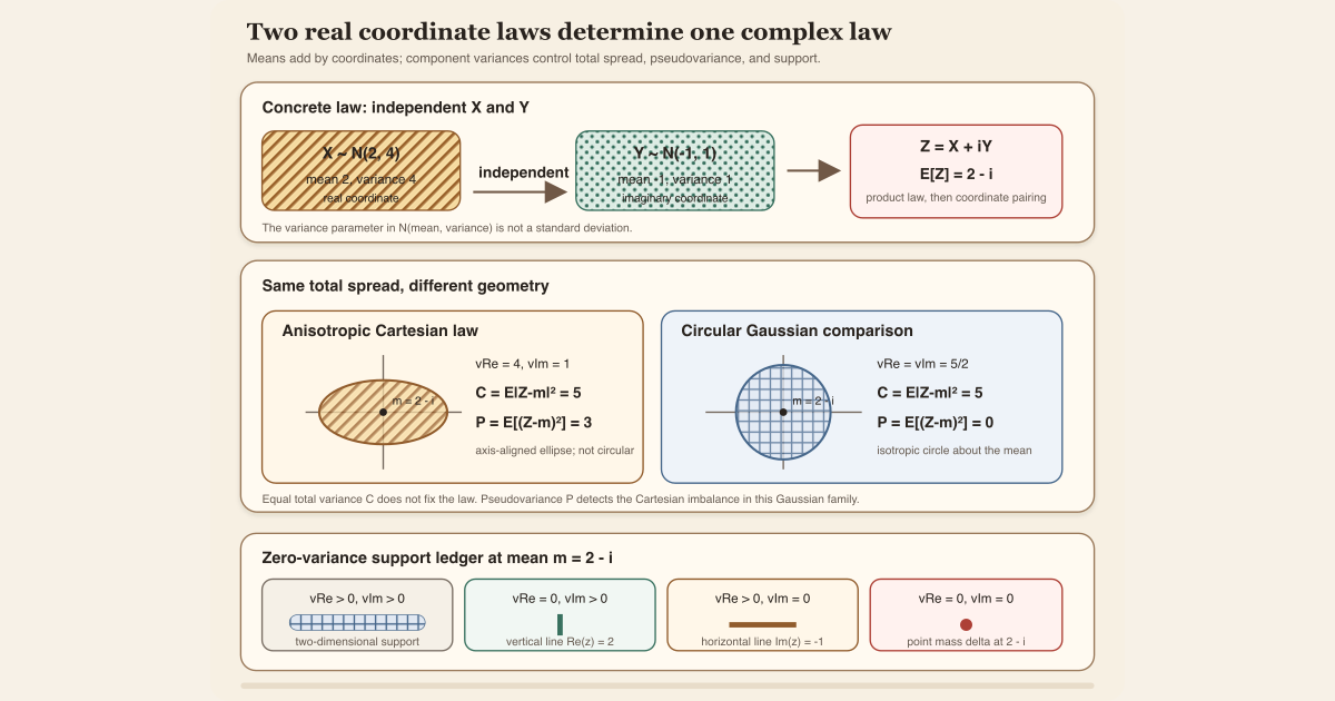
A Cartesian complex Gaussian law builds a probability measure on \(\mathbb C\) from two independent real Gaussian coordinates. It records the real-part variance and imaginary-part variance separately instead of hiding both behind the ambiguous phrase “complex variance.”

\[ X\sim N(m_{\mathrm R},v_{\mathrm R}), \qquad Y\sim N(m_{\mathrm I},v_{\mathrm I}), \]

and \(X\) and \(Y\) are independent, then

\[ Z=X+iY \]

has Cartesian complex Gaussian mean \(m=m_{\mathrm R}+im_{\mathrm I}\) and component variances \((v_{\mathrm R},v_{\mathrm I})\).

The component laws are necessary, but they are not enough by themselves. Independence fixes the joint product law.

A fully computed anisotropic example

Take independent real random variables

\[ X\sim N(2,4), \qquad Y\sim N(-1,1), \]

where the second parameter is the variance. Define

\[ Z=X+iY. \]

Linearity of expectation gives

\[ \begin{aligned} \mathbb E[Z] &=\mathbb E[X]+i\mathbb E[Y]\\ &=2-i. \end{aligned} \]

Thus the complex mean is

\[ m=2-i. \]

Center the real coordinates:

\[ U=X-2, \qquad V=Y+1. \]

Then \(Z-m=U+iV\), with

\[ \mathbb E[U]=\mathbb E[V]=0, \qquad \mathbb E[U^2]=4, \qquad \mathbb E[V^2]=1. \]

The expected centered squared magnitude is

\[ \begin{aligned} C &=\mathbb E\!\left[(Z-m)\overline{(Z-m)}\right]\\ &=\mathbb E|Z-m|^2\\ &=\mathbb E[U^2+V^2]\\ &=4+1\\ &=5. \end{aligned} \]

Many texts call \(C\) the complex covariance or complex variance. This page uses the explicit formula because the word “variance” alone does not determine whether it means a component variance or the total \(C\).

Pseudovariance detects the imbalance

The pseudovariance, also called the relation or complementary covariance, is

\[ P=\mathbb E[(Z-m)^2]. \]

Expand the square:

\[ (U+iV)^2=U^2-V^2+2iUV. \]

Independence and centering give

\[ \mathbb E[UV]=\mathbb E[U]\mathbb E[V]=0. \]

Therefore

\[ \begin{aligned} P &=\mathbb E[U^2]-\mathbb E[V^2] +2i\mathbb E[UV]\\ &=4-1+0\\ &=3. \end{aligned} \]

The two complex second-order quantities are different:

\[ C=v_{\mathrm R}+v_{\mathrm I}, \qquad P=v_{\mathrm R}-v_{\mathrm I} \]

for an independent Cartesian pair. \(C\) records total spread. \(P\) records the difference between the two coordinate spreads.

For a general centered real pair that is not independent, the formula becomes

\[ P=v_{\mathrm R}-v_{\mathrm I} +2i\,\operatorname{Cov}(X,Y). \]

The Cartesian product law sets that cross-covariance to zero.

Anisotropic versus circular with the same total spread

The worked law has

\[ (v_{\mathrm R},v_{\mathrm I})=(4,1). \]

Its standard deviations are \(2\) horizontally and \(1\) vertically, so its constant-density contours are axis-aligned ellipses. Its nonzero pseudovariance \(P=3\) records that anisotropy.

Now keep the same mean \(m=2-i\) and the same total variance \(C=5\), but use

\[ v_{\mathrm R}=v_{\mathrm I}=\frac52. \]

Then

\[ C=\frac52+\frac52=5, \qquad P=\frac52-\frac52=0. \]

The centered Gaussian law now has circular contours and is invariant under every complex phase rotation about its mean:

\[ e^{i\theta}(Z-m)\stackrel{d}{=}Z-m. \]

The two laws have the same mean and the same total \(C\), yet they are not the same law. The pseudovariance distinguishes them.

Independent real Gaussian X with mean two and variance four and Y with mean minus one and variance one combine into Z equals X plus iY with mean two minus i. An ellipse displays total complex variance five and pseudovariance three. A circular comparison with component variances five halves and five halves has the same total five and pseudovariance zero. Four lower cards show full-plane, vertical-line, horizontal-line, and point-mass support branches. — FigureFinding: \(X\sim N(2,4)\) and \(Y\sim N(-1,1)\), independently, give \(Z=X+iY\) with \(\mathbb E[Z]=2-i\), total centered squared magnitude \(C=\mathbb E|Z-(2-i)|^2=5\), and pseudovariance \(P=\mathbb E[(Z-(2-i))^2]=3\). Replacing component variances \((4,1)\) by \((5/2,5/2)\) keeps \(C=5\) but changes \(P\) to zero and makes the centered Gaussian circularly symmetric. The support ledger shows why zero variances must be handled as line or point measures rather than by a positive planar density. Patterns distinguish coordinate roles and geometry without relying on color.

The exact measure construction

Let \(\gamma_{a,v}\) denote the real Gaussian probability measure with mean \(a\) and variance \(v\). Define

\[ \Phi:\mathbb R\times\mathbb R\longrightarrow\mathbb C, \qquad \Phi(x,y)=x+iy. \]

The Cartesian complex Gaussian measure is

\[ \Gamma^{\mathrm{cart}}_{m;v_{\mathrm R},v_{\mathrm I}} {}= \Phi_*\left( \gamma_{m_{\mathrm R},v_{\mathrm R}} \otimes \gamma_{m_{\mathrm I},v_{\mathrm I}} \right). \]

The product symbol \(\otimes\) fixes independence . The pushforward through \(\Phi\) then changes the representation from a real coordinate pair to one complex number.

Reading the measure back through the coordinate maps recovers

\[ \operatorname{Re}Z\sim\gamma_{m_{\mathrm R},v_{\mathrm R}}, \qquad \operatorname{Im}Z\sim\gamma_{m_{\mathrm I},v_{\mathrm I}}. \]

More strongly, the joint law is the product:

\[ \mathcal L(\operatorname{Re}Z,\operatorname{Im}Z) {}= \gamma_{m_{\mathrm R},v_{\mathrm R}} \otimes \gamma_{m_{\mathrm I},v_{\mathrm I}}. \]

This is an exact probability law , not an estimate from a sample cloud.

Gaussian marginals do not prove independence

Let \(G\sim N(0,1)\), and set

\[ X=G, \qquad Y=G. \]

Both \(X\) and \(Y\) have the standard real Gaussian marginal law, but they are perfectly dependent. The pair \((X,Y)\) lies on the diagonal line \(\{(x,x):x\in\mathbb R\}\), not under the product of two Gaussian measures. The complex variable

\[ Z=(1+i)G \]

is supported on a slanted line. It is a valid real two-dimensional Gaussian variable, but it is not the Cartesian independent-coordinate law with component variances \(1\) and \(1\).

Thus the correct constructor needs three inputs:

the exact law of \(X\);
the exact law of \(Y\); and
their independence.

Zero covariance would not replace independence for arbitrary non-Gaussian variables. In the present construction, the full product law is the primary fact.

Density and support, including every zero branch

When both component variances are positive, the law has planar density

\[ f(x+iy) {}= \frac{1}{2\pi\sqrt{v_{\mathrm R}v_{\mathrm I}}} \exp\!\left( -\frac{(x-m_{\mathrm R})^2}{2v_{\mathrm R}} -\frac{(y-m_{\mathrm I})^2}{2v_{\mathrm I}} \right). \]

For the anisotropic example,

\[ f(x+iy) {}= \frac1{4\pi} \exp\!\left( -\frac{(x-2)^2}{8} -\frac{(y+1)^2}{2} \right). \]

The equal-variance comparison instead has

\[ f_{\mathrm{circ}}(x+iy) {}= \frac1{5\pi} \exp\!\left( -\frac{(x-2)^2+(y+1)^2}{5} \right). \]

These density formulas are valid only when both variances are positive. The measure construction remains meaningful in all boundary cases:

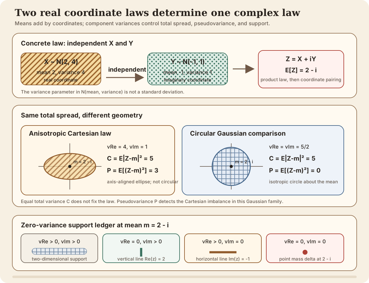
Component variances	Exact support geometry
\(v_{\mathrm R}\gt0,\ v_{\mathrm I}\gt0\)	two-dimensional plane, with an elliptical density
\(v_{\mathrm R}=0,\ v_{\mathrm I}\gt0\)	vertical line \(\operatorname{Re}z=m_{\mathrm R}\)
\(v_{\mathrm R}\gt0,\ v_{\mathrm I}=0\)	horizontal line \(\operatorname{Im}z=m_{\mathrm I}\)
\(v_{\mathrm R}=v_{\mathrm I}=0\)	point mass \(\delta_m\)

At \(v_{\mathrm R}=0\), the real Gaussian coordinate equals \(m_{\mathrm R}\) almost surely. At \(v_{\mathrm I}=0\), the imaginary coordinate equals \(m_{\mathrm I}\) almost surely. When both vanish, \(Z=m\) almost surely.

A line-supported or point-supported law is singular with respect to planar area. Substituting zero into the positive density formula is not a legitimate shortcut.

Properness and circularity

A second-order complex variable is called proper when its centered pseudovariance is zero. For the independent Cartesian Gaussian family,

\[ P=0 \quad\Longleftrightarrow\quad v_{\mathrm R}=v_{\mathrm I}. \]

Equal component variances make the complete centered Gaussian law isotropic, so properness and circular symmetry agree in this family. They are not synonyms in arbitrary non-Gaussian settings: pseudovariance is only second-order information, while circular symmetry is an equality of complete laws.

The center matters. A nonzero-mean law may be circular about \(m\), meaning its centered variable is phase invariant, without being invariant under rotations about the origin.

The project’s current Lean module formalizes the product law, coordinate marginals, independence, integrability, mean, and double-zero Dirac branch. It does not yet formalize the planar density, \(C\), \(P\), properness, or circular symmetry. Those interpretations remain explicit mathematical boundaries rather than claims attributed to the checker.

In Lean: the complete law predicate

One idea, three languages Read across, then read the syntax map

A human says

Under the source measure P, Z has complex mean m, real-coordinate variance vRe, imaginary-coordinate variance vIm, and the product dependence structure built into the Cartesian law.

On paper

\(\mathcal L_P(Z)=\Gamma^{\mathrm{cart}}_{m;v_{\mathrm R},v_{\mathrm I}}.\)

In Lean

hZ : NonlinearDynamics.Random.HasCartesianComplexGaussianLaw Z m vRe vIm P

Syntax map

Z : Ω → ℂ is the complex random variable.
m : ℂ is the complex mean parameter. Its fields m.re and m.im parameterize the real coordinate laws.
vRe vIm : ℝ≥0 are nonnegative real numbers. They are coordinate variances, not standard deviations and not a single total complex variance.
P : Measure Ω is the source measure.
HasCartesianComplexGaussianLaw Z m vRe vIm P unfolds to an exact HasLaw statement for the pushed-forward product measure.
hZ is a human-chosen name for evidence of the entire statement. From it, hZ.real_hasLaw, hZ.imag_hasLaw, and hZ.indep_re_im recover the component facts.
hZ.mean_eq proves the typed equation ∫ ω, Z ω ∂P = m, the Lean counterpart of \(\mathbb E[Z]=m\).

The constructor exposes independence instead of inferring it from marginals:

One idea, three languages Read across, then read the syntax map

A human says

If X and Y have the requested exact real Gaussian laws and are independent, then omega mapped to X(omega) plus i times Y(omega) has the requested Cartesian complex Gaussian law.

On paper

\(X\sim N(m_{\mathrm R},v_{\mathrm R}),\ Y\sim N(m_{\mathrm I},v_{\mathrm I}),\ X\perp Y\Longrightarrow X+iY\sim\Gamma^{\mathrm{cart}}_{m;v_{\mathrm R},v_{\mathrm I}}.\)

In Lean

NonlinearDynamics.Random.HasCartesianComplexGaussianLaw.of_indep_re_im hX hY hXY

Syntax map

hX : HasRealGaussianLaw X m.re vRe P is the exact real-part law.
hY : HasRealGaussianLaw Y m.im vIm P is the exact imaginary-part law.
hXY : IndepFun X Y P is the separate dependence certificate.
The conclusion is a law for fun ω ↦ X ω + Y ω * Complex.I.
Complex.I is Lean’s imaginary unit \(i\).
A human can first type #check with the fully qualified theorem name, then apply it to the three named proof objects as shown.

Exact project excerpts

The checked measure and predicate definitions are:

noncomputable def cartesianComplexGaussian (m : ℂ) (vRe vIm : ℝ≥0) :
    Measure ℂ :=
  ((gaussianReal m.re vRe).prod (gaussianReal m.im vIm)).map
    Complex.equivRealProdCLM.symm

def HasCartesianComplexGaussianLaw (Z : Ω → ℂ) (m : ℂ)
    (vRe vIm : ℝ≥0) (P : Measure Ω) : Prop :=
  HasLaw Z (cartesianComplexGaussian m vRe vIm) P

The real-linear equivalence Complex.equivRealProdCLM.symm sends a coordinate pair to its complex number. The product measure supplies both marginals and their independence before that pushforward.

The mean theorem is also checked directly:

theorem mean_eq (hZ : HasCartesianComplexGaussianLaw Z m vRe vIm P) :
    ∫ ω, Z ω ∂P = m := by
  apply Complex.ext
  · have hRealIntegral :
        ∫ ω, (Z ω).re ∂P = (∫ ω, Z ω ∂P).re := by
      simpa only [RCLike.re_to_complex] using integral_re hZ.integrable
    rw [← hRealIntegral]
    exact hZ.real_hasLaw.mean_eq
  · have hImagIntegral :
        ∫ ω, (Z ω).im ∂P = (∫ ω, Z ω ∂P).im := by
      simpa only [RCLike.im_to_complex] using integral_im hZ.integrable
    rw [← hImagIntegral]
    exact hZ.imag_hasLaw.mean_eq

The proof uses complex extensionality: two complex numbers are equal after their real and imaginary parts are proved equal. Each coordinate equality then comes from the corresponding exact real Gaussian law.

The double-zero boundary is a measure identity and an almost-everywhere random-variable identity:

theorem cartesianComplexGaussian_zero_variances (m : ℂ) :
    cartesianComplexGaussian m 0 0 = Measure.dirac m := by
  unfold cartesianComplexGaussian
  simp only [gaussianReal_zero_var, Measure.dirac_prod_dirac]
  have hMean : Complex.equivRealProdCLM.symm (m.re, m.im) = m := by
    apply Complex.ext <;> simp
  rw [Measure.map_dirac, hMean]

theorem ae_eq_const_of_variances_zero
    (hZ : HasCartesianComplexGaussianLaw Z m 0 0 P) :
    Z =ᵐ[P] fun _ ↦ m := by
  apply ProbabilityTheory.HasLaw.ae_eq_of_dirac
  simpa only [HasCartesianComplexGaussianLaw,
    cartesianComplexGaussian_zero_variances] using hZ

The conclusion is almost everywhere because a probability law cannot detect changes made on a \(P\)-null set. Consistently, HasLaw asks only for almost-everywhere measurability; ordinary measurability would still not upgrade equality in law with a Dirac mass to pointwise equality everywhere.

Standalone tutorial: arithmetic worksheet

Standalone tutorial. This worksheet imports only Std and computes exact rational ledger values. It does not import Mathlib or the project, and it does not prove Gaussianity or independence.

Save the following as ComplexGaussianMomentsScratch.lean:

import Std

structure CartesianMomentLedger where
  meanRe : Rat
  meanIm : Rat
  varRe : Rat
  varIm : Rat
deriving Repr

def complexMean (L : CartesianMomentLedger) : Rat × Rat :=
  (L.meanRe, L.meanIm)

def totalVariance (L : CartesianMomentLedger) : Rat :=
  L.varRe + L.varIm

def pseudovariance (L : CartesianMomentLedger) : Rat :=
  L.varRe - L.varIm

def anisotropic : CartesianMomentLedger :=
  { meanRe := 2, meanIm := -1, varRe := 4, varIm := 1 }

def circularSameTotal : CartesianMomentLedger :=
  { meanRe := 2, meanIm := -1,
    varRe := (5 : Rat) / 2, varIm := (5 : Rat) / 2 }

#eval complexMean anisotropic
#eval totalVariance anisotropic
#eval pseudovariance anisotropic
#eval totalVariance circularSameTotal
#eval pseudovariance circularSameTotal

Run it with:

elan run leanprover/lean4:v4.32.0 lean ComplexGaussianMomentsScratch.lean

The exact outputs should be the pair \((2,-1)\), then \(5\), \(3\), \(5\), and \(0\). The worksheet checks the arithmetic ledger used in the example. The project declarations below carry the measure-theoretic content.

Project-source workflow

Try it in the repository NonlinearDynamics/Random/ComplexGaussian.lean

Full project check. This uses the repository’s pinned Lean and Mathlib dependencies and may require substantial disk space and memory. The authoritative source is formalization/NonlinearDynamics/Random/ComplexGaussian.lean. Create a temporary project worksheet containing:

import NonlinearDynamics.Random.ComplexGaussian

#check NonlinearDynamics.Random.cartesianComplexGaussian
#check NonlinearDynamics.Random.cartesianComplexGaussian_map_re
#check NonlinearDynamics.Random.cartesianComplexGaussian_map_im
#check NonlinearDynamics.Random.cartesianComplexGaussian_zero_variances
#check NonlinearDynamics.Random.HasCartesianComplexGaussianLaw
#check NonlinearDynamics.Random.HasCartesianComplexGaussianLaw.jointHasLaw
#check NonlinearDynamics.Random.HasCartesianComplexGaussianLaw.real_hasLaw
#check NonlinearDynamics.Random.HasCartesianComplexGaussianLaw.imag_hasLaw
#check NonlinearDynamics.Random.HasCartesianComplexGaussianLaw.indep_re_im
#check NonlinearDynamics.Random.HasCartesianComplexGaussianLaw.mean_eq
#check NonlinearDynamics.Random.HasCartesianComplexGaussianLaw.ae_eq_const_of_variances_zero
#check NonlinearDynamics.Random.HasCartesianComplexGaussianLaw.of_indep_re_im

Each #check asks the pinned elaborator for an exact declaration type. The commands do not establish a planar density, pseudovariance, or circular symmetry theorem, because those declarations are not yet in this module. The full-project command below checks the complete source module with the repository’s pinned dependencies installed.

Full project check, from the repository root

cd formalization
lake env lean -DwarningAsError=true NonlinearDynamics/Random/ComplexGaussian.lean

Resource note: this exact file uses the repository's pinned Lean and Mathlib dependencies. Initial project setup can require substantial disk space and build time. For a lightweight first step on macOS or Linux, use the page's standalone Lean-core or Std tutorial.

Distinctions and failure modes

Tempting shortcut	What is wrong	Correct repair
“Both marginals are Gaussian, so the pair is Cartesian”	Marginals do not determine dependence	Prove the joint product law or independence
“Complex variance is \(v_{\mathrm R}\)”	One component variance omits the other coordinate	State \(v_{\mathrm R}\), \(v_{\mathrm I}\), \(C\), or \(P\) explicitly
“Total variance \(C\) determines the ellipse”	\((4,1)\) and \((5/2,5/2)\) both give \(C=5\)	Record pseudovariance or the full covariance matrix
“Zero pseudovariance always means circular symmetry”	Pseudovariance is only second-order data outside Gaussian laws	Prove full phase invariance when circularity is required
“A circular centered law is invariant about the origin”	A nonzero mean moves the center of rotation	State whether the variable is centered
“The planar density works at zero variance”	A zero component produces singular line support	Use the measure definition and its degenerate branch
“Both zero variances mean pointwise equality everywhere”	The law interface concludes equality almost everywhere	Use the a.e. theorem or add representative assumptions
“HasLaw means ordinary measurability”	The interface stores almost-everywhere measurability	Keep stronger measurability as a separate hypothesis when needed
“Cartesian Gaussian already means GUE entry”	A matrix ensemble also needs dimension scaling, indexing, reflection, and cross-coordinate independence	Publish a normalization ledger before assembly

Where to continue

Read Gaussian distribution for each real coordinate, independence for the product law, and variance for the scalar second-moment parameter. The independent Cartesian complex Gaussian family entry lifts this law to indexed coordinates.

Complex Gaussian Coordinates and Geometry develops the density and symmetry discussion. Finite Product Probability Spaces and Independent Gaussian Fields explains why independence inside each pair differs from independence across a whole family.

References

Mathlib contributors. Gaussian distributions over the reals, Mathlib 4 documentation. This official API defines the exact coordinate measures and their zero-variance Dirac branches.

Mathlib contributors. Law of a random variable, Mathlib 4 documentation. This is the official source for the pushforward and almost-everywhere measurability fields carried by HasLaw.

F. D. Neeser and J. L. Massey. Proper Complex Random Processes with Applications to Information Theory, IEEE Transactions on Information Theory 39 (1993), 1293-1302. This primary source develops covariance, pseudocovariance, and properness.

Bernard Picinbono. Second-Order Complex Random Vectors and Normal Distributions, IEEE Transactions on Signal Processing 44 (1996), 2637-2640. This primary source distinguishes covariance and relation information for complex normal laws.

Nonlinear Dynamics in Lean contributors. ComplexGaussian.lean, the checked project source for the exact Cartesian law, coordinate product structure, mean, integrability, independence, and zero-variance boundary.