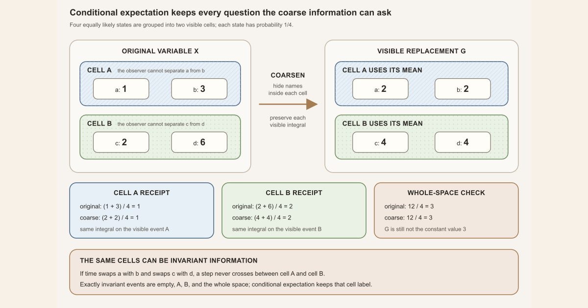
Start with four equally likely states
Let
\[ \Omega=\{a,b,c,d\}. \]Every subset is an event , and every event is measurable. Give each state probability \(1/4\). This is the uniform probability measure \(\mathbb P\):
\[ \mathbb P(\{a\}) =\mathbb P(\{b\}) =\mathbb P(\{c\}) =\mathbb P(\{d\}) =\frac14. \]Define the real random variable \(X:\Omega\to\mathbb R\) by
| State \(\omega\) | \(a\) | \(b\) | \(c\) | \(d\) |
|---|---|---|---|---|
| \(X(\omega)\) | \(1\) | \(3\) | \(2\) | \(6\) |
Now suppose an observer learns only which of these two cells contains the state:
\[ A=\{a,b\}, \qquad B=\{c,d\}. \]The observer’s information is the four-event sigma algebra
\[ \mathcal G=\{\varnothing,A,B,\Omega\}. \]A sigma algebra is a collection of measurable yes-or-no questions that contains the empty event and is closed under complements and countable unions. Here \(\mathcal G\) distinguishes \(A\) from \(B\), but not \(a\) from \(b\), or \(c\) from \(d\). The measurable-space entry develops those closure rules from the beginning.
Calculate the coarse value cell by cell
Call the information-visible replacement \(G\). A real function measurable with respect to \(\mathcal G\) must be constant on each cell. Write
\[ G(a)=G(b)=u, \qquad G(c)=G(d)=v. \]Conditional expectation chooses \(u\) and \(v\) so replacing \(X\) by \(G\) does not change the integral on any event the observer can see.
On the first cell,
\[ \int_A G\,d\mathbb P =\frac14u+\frac14u =\int_A X\,d\mathbb P =\frac14(1)+\frac14(3) =1. \]Thus \(u/2=1\), so \(u=2\). On the second cell,
\[ \int_B G\,d\mathbb P =\frac14v+\frac14v =\int_B X\,d\mathbb P =\frac14(2)+\frac14(6) =2. \]Thus \(v/2=2\), so \(v=4\). One version of the conditional expectation is
\[ G=\mathbb E_{\mathbb P}[X\mid\mathcal G], \qquad (G(a),G(b),G(c),G(d))=(2,2,4,4). \]There are only four \(\mathcal G\)-measurable events, so the complete defining test fits in one table:
| Visible event \(S\) | \(\int_S X\,d\mathbb P\) | \(\int_S G\,d\mathbb P\) |
|---|---|---|
| \(\varnothing\) | \(0\) | \(0\) |
| \(A\) | \((1+3)/4=1\) | \((2+2)/4=1\) |
| \(B\) | \((2+6)/4=2\) | \((4+4)/4=2\) |
| \(\Omega\) | \((1+3+2+6)/4=3\) | \((2+2+4+4)/4=3\) |
The two cell rows determine the two values. The empty row is automatic, and the whole-space row follows by adding the \(A\) and \(B\) rows. Listing all four rows makes the phrase “every visible event” literal and checkable.
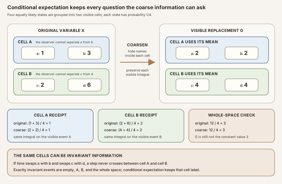
Compare the fine variable, the coarse view, and the global mean
The original variable, conditional expectation, and ordinary expectation answer different questions:
| Object | Values on \(a,b,c,d\) | Information retained |
|---|---|---|
| \(X\) | \((1,3,2,6)\) | Exact state |
| \(\mathbb E[X\mid\mathcal G]\) | \((2,2,4,4)\) | Cell \(A\) or \(B\) |
| Constant \(\mathbb E[X]\) | \((3,3,3,3)\) | No state information |
The global expectation is
\[ \mathbb E_{\mathbb P}[X] =\frac{1+3+2+6}{4} =3. \]Although \(G\) has the same global expectation, it is not the constant function \(3\). On \(A\),
\[ \int_A X\,d\mathbb P =1 =\int_A G\,d\mathbb P, \qquad \int_A 3\,d\mathbb P =\frac32. \]Matching only the whole-space integral discards too much information. Conditional expectation must match \(X\) on every event in the chosen sigma algebra.
The endpoint information fields calibrate the construction:
- For the full sigma algebra, \(X\) is already visible, so \(\mathbb E[X\mid\mathcal F]=X\) almost everywhere.
- For the bottom sigma algebra \(\{\varnothing,\Omega\}\), every visible real function is constant. On a probability space that constant is \(\mathbb E[X]=3\).
- For the intermediate field \(\mathcal G\), the answer keeps the cell label and discards only variation inside each cell.
Equal weights made the cell values arithmetic means. With unequal masses they are weighted means. If \(a\) and \(b\) have masses \(1/8\) and \(3/8\), the \(A\)-cell value becomes
\[ \frac{(1/8)1+(3/8)3}{1/8+3/8} =\frac52, \]not \(2\). The answer depends on both the sigma algebra and the measure.
The general definition
Let \((\Omega,\mathcal F,\mu)\) be a measure space. The sigma algebra \(\mathcal F\) specifies the ambient measurable events, and the measure \(\mu\) assigns them mass. Let \(\mathcal G\le\mathcal F\) be a smaller sigma algebra, meaning every \(\mathcal G\)-measurable event is also \(\mathcal F\)-measurable. Finally, let \(f:\Omega\to\mathbb R\) be integrable .
A function \(g:\Omega\to\mathbb R\) is a version of \(\mathbb E_\mu[f\mid\mathcal G]\) when:
\(g\) is measurable using only \(\mathcal G\), up to modification on a \(\mu\)-null set;
\(g\) is integrable; and
every \(\mathcal G\)-measurable event \(S\) has the same restricted integral under \(g\) and \(f\):
\[ \int_S g\,d\mu=\int_S f\,d\mu. \]
The first item forbids \(g\) from using invisible distinctions. The second controls its size. The third preserves every weighted question visible to the chosen information field.
The characterization determines \(g\) only almost everywhere , abbreviated a.e. Two functions are a.e. equal when the event on which they differ is a null set , an event of measure zero. Changing an integrable function on a null set changes none of its measurable-set integrals.
The notation \(\mathbb E[f\mid\mathcal G]\) conditions on an entire sigma algebra, not one event. An expression such as \(\mathbb E[f\mid A]\) uses a related event-conditioning convention and needs its own normalization and positive-probability assumptions.
Almost-everywhere uniqueness leaves representatives
In the four-state example every singleton has probability \(1/4\). Its only null event is \(\varnothing\), so a.e.-equal functions are actually equal at all four states. That is why the table produces one pointwise answer.
Now append a fifth state \(z\) of probability zero and let \(\{z\}\) be its own visible cell. Two candidates can agree with \((2,2,4,4)\) on \(a,b,c,d\) while taking \(0\) and \(99\) at \(z\). They are different ordinary functions, but they are equal a.e. and represent the same conditional expectation.
Mathlib returns an ordinary function because later expressions evaluate it at
an outcome. Its MeasureTheory.condExp is a selected
representative, and identification theorems normally conclude with Lean’s
a.e.-equality relation rather than literal function equality.
Mathlib’s definition is total. It returns the zero function when the requested smaller measurable space is not below the ambient one, when the trimmed measure is not sigma-finite, or when the input is not integrable. This makes the Lean term meaningful outside the usual hypotheses. It does not make the usual measurability and integral identities true without those hypotheses.
In Lean: name the selected representative
Mathlib writes conditional expectation as
MeasureTheory.condExp 𝓖 μ f and provides the notation
μ[f | 𝓖].
g =ᵐ[μ] μ[f | 𝓖]g =ᵐ[μ] his equality almost everywhere with respect toμ, not literal function equality.- The first
μ, inside=ᵐ[μ], supplies the measure for the exceptional null set. - The second
μ, before the bracket, supplies the measure for the conditional expectation. fis the original integrable function.- The vertical bar in
μ[f | 𝓖]is read “given 𝓖.” 𝓖is aMeasurableSpace Ω, the Lean structure storing the selected sigma algebra on the outcome type.
In Lean: preserve every visible-set integral
∫ x in S, g x ∂μ = ∫ x in S, f x ∂μ∫ x in S, … ∂μis a set integral, restricted toSand taken with respect toμ.g xandf xare ordinary function applications.- The separate premise
MeasurableSet[𝓖] Ssays thatSis visible to the selected sigma algebra. setIntegral_condExpproves the identity for Mathlib’s selected representative under the sub-sigma-algebra, sigma-finiteness, and integrability hypotheses.ae_eq_condExp_of_forall_setIntegral_eqsays that an a.e. \(\mathcal G\)-measurable candidate with the local integrability and every visible-set identity is a.e. equal toμ[f | 𝓖].
The exact uniqueness interface used by the project is:
theorem ae_eq_condExp_of_forall_setIntegral_eq
    (h𝓖 : 𝓖 ≤ 𝓕) [SigmaFinite (μ.trim h𝓖)]
    (hf : Integrable f μ)
    (hg_int : ∀ S, MeasurableSet[𝓖] S → μ S < ∞ →
      IntegrableOn g S μ)
    (hg_eq : ∀ S, MeasurableSet[𝓖] S → μ S < ∞ →
      ∫ x in S, g x ∂μ = ∫ x in S, f x ∂μ)
    (hgm : AEStronglyMeasurable[𝓖] g μ) :
    g =ᵐ[μ] μ[f | 𝓖]
Here μ.trim h𝓖 is the measure viewed on the smaller measurable
space. The general theorem supports sigma-finite measures, so its local
premises mention finite-measure visible sets. The project works under
IsFiniteMeasure μ; global integrability then supplies those local
obligations. Finite measure does not mean probability measure.
A tiny standalone Lean worksheet a human can type
Standalone tutorial. This worksheet checks the integer numerators behind the four-state example. Dividing every sum by the common denominator \(4\) gives the probability integrals. It does not define Mathlib measures, sigma algebras, conditional expectation, or a.e. equality.
Save it as ConditionalExpectationFiniteScratch.lean:
import Std

inductive Atom where
  | a | b | c | d
deriving Repr, DecidableEq

def atoms : List Atom := [.a, .b, .c, .d]
def cellA : List Atom := [.a, .b]
def cellB : List Atom := [.c, .d]

def value : Atom → Int
  | .a => 1
  | .b => 3
  | .c => 2
  | .d => 6

def coarseValue : Atom → Int
  | .a => 2
  | .b => 2
  | .c => 4
  | .d => 4

def sumOn (event : List Atom) (h : Atom → Int) : Int :=
  (event.map h).sum

#eval atoms.map value
#eval atoms.map coarseValue
#eval [sumOn cellA value, sumOn cellA coarseValue]
#eval [sumOn cellB value, sumOn cellB coarseValue]
#eval [sumOn atoms value, sumOn atoms coarseValue]

example : sumOn cellA value = sumOn cellA coarseValue := by decide
example : sumOn cellB value = sumOn cellB coarseValue := by decide
example : sumOn atoms value = 12 := by decide
example : sumOn atoms coarseValue = 12 := by decide
example : coarseValue .a ≠ value .a := by decide
example : coarseValue .a ≠ 3 := by decide
From the directory containing the file, type:
source "$HOME/.elan/env"
elan run leanprover/lean4:v4.32.0 lean ConditionalExpectationFiniteScratch.lean
This exact worksheet was executed successfully with Lean 4.32.0 while editing
this page. The evaluations printed [1, 3, 2, 6],
[2, 2, 4, 4], then [4, 4], [8, 8],
and [12, 12]. The last pair gives global expectation
\(12/4=3\). The final two example commands ask Lean’s kernel to
check proof terms stating that the coarse value at \(a\) is neither \(X(a)\)
nor the constant global mean. This command is
suitable for an ordinary Mac or Linux machine because it imports only
Std.
The invariant-sigma-algebra connection
Read the same example dynamically. Define one time step \(T:\Omega\to\Omega\) by
\[ T(a)=b, \quad T(b)=a, \quad T(c)=d, \quad T(d)=c. \]The uniform probability measure is preserved. An event is exactly unchanged by one-step preimage precisely when it is a union of the two cycles. Therefore the exact invariant sigma algebra is
\[ \mathcal I_T=\{\varnothing,A,B,\Omega\}=\mathcal G. \]Starting from \(a\) or \(b\), observed values alternate \(1,3,1,3,\ldots\), whose averages tend to \(2\). Starting from \(c\) or \(d\), they alternate \(2,6,2,6,\ldots\), whose averages tend to \(4\). Thus this finite model has
\[ \lim_{n\to\infty} \frac1n\sum_{j=0}^{n-1}X(T^j\omega) =\mathbb E_{\mathbb P}[X\mid\mathcal I_T](\omega) \]at every state.
The example is nonergodic: \(A\) and \(B\) are invariant events of probability \(1/2\). The limit may therefore take two values. Ergodicity is an additional hypothesis that collapses invariant information modulo null sets and can turn the target into one a.e.-constant normalized space average. Conditional expectation onto an invariant field is not automatically constant.
The project theorem allows any finite measure, any measure-preserving self-map, and any integrable real observable. Its conclusion is a.e., not everywhere.
∀ᵐ ω ∂μ, Tendsto (fun n ↦ birkhoffAverage ℝ T f n ω) atTop (nhds (μ[f | MeasurableSpace.invariants T] ω))∀ᵐ ω ∂μreads “for almost every outcomeωwith respect toμ.”fun n ↦ …is the sequence indexed by horizonn.birkhoffAverage ℝ T f n ωaverages along the firstniterates ofTfromω.Tendsto … atTopsays the sequence converges asngrows without bound.nhds yis the neighborhood filter at the proposed limity.MeasurableSpace.invariants Tis Mathlib’s exact invariant sigma algebra. The theorem does not replace it by bottom without a later ergodic rigidity result.
Why the project limit qualifies
Random-matrix-theory milestone 27 (RMT-27) starts from the preceding milestone’s a.e. convergence of finite Birkhoff averages. Convergence alone does not identify the target. RMT-27 then verifies three separate conditional-expectation obligations.
- Invariant measurability. A prefix-shift argument makes the selected
total
birkhoffLimit T fliterally invariant, including on its divergent fallback branch. - Integrability. Pointwise convergence alone is insufficient. Uniform integrability of the Cesaro averages and finite-measure Vitali convergence supply \(L^1\) convergence and an integrable limit.
- Visible-set identities. On an exactly invariant measurable event, measure preservation keeps every orbit translate’s integral equal to the original integral. \(L^1\) convergence passes that identity to the limit.
Mathlib’s uniqueness theorem then gives:
theorem birkhoffLimit_ae_eq_condExp
    [IsFiniteMeasure μ]
    (hT : MeasurePreserving T μ μ) (hf : Integrable f μ) :
    birkhoffLimit T f =ᵐ[μ]
      μ[f | MeasurableSpace.invariants T]
Combining identification with convergence gives:
theorem ae_tendsto_birkhoffAverage_condExp
    [IsFiniteMeasure μ]
    (hT : MeasurePreserving T μ μ) (hf : Integrable f μ) :
    ∀ᵐ ω ∂μ,
      Tendsto (fun n ↦ birkhoffAverage ℝ T f n ω) atTop
        (nhds (μ[f | MeasurableSpace.invariants T] ω))
No probability, ergodicity, injectivity, surjectivity, or invertibility assumption occurs in those signatures. The zero measure is allowed; there the a.e. conclusion is vacuous. These are checked theorem properties, not conclusions inferred from the finite example.
Try the exact declarations in the project
Full project check. This uses the repository’s pinned Lean and Mathlib dependencies and may require substantial disk space and memory. Create a temporary project worksheet containing:
import NonlinearDynamics.Random.RandomCocycles.PointwiseBirkhoffLimit

open MeasureTheory Set Filter Function
open NonlinearDynamics.Random.RandomCocycles

universe uΩ

variable {Ω : Type uΩ} [MeasurableSpace Ω]
variable {μ : Measure Ω} {𝓖 : MeasurableSpace Ω}
variable {T : Ω → Ω} {f g : Ω → ℝ}

#check (μ[f | 𝓖])
#check MeasureTheory.stronglyMeasurable_condExp
#check MeasureTheory.integrable_condExp
#check MeasureTheory.setIntegral_condExp
#check MeasureTheory.ae_eq_condExp_of_forall_setIntegral_eq
#check MeasureTheory.condExp_congr_ae
#check measurable_birkhoffLimit_invariants
#check setIntegral_birkhoffLimit_eq
#check birkhoffLimit_ae_eq_condExp
#check ae_tendsto_birkhoffAverage_condExp
Each #check asks the pinned elaborator for an exact declaration
type. The full-project command below checks the authoritative RMT-27 module;
it is separate from the standalone Std tutorial.
cd formalization
lake env lean -DwarningAsError=true NonlinearDynamics/Random/RandomCocycles/PointwiseBirkhoffLimit.lean
Resource note: this exact file uses the repository's
pinned Lean and Mathlib dependencies. Initial project setup can require
substantial disk space and build time. For a lightweight first step on
macOS or Linux, use the page's standalone Lean-core or Std
tutorial.
Boundaries and nonclaims
- Global equality is too weak. Matching \(\int_\Omega g\,d\mu=\int_\Omega f\,d\mu\) does not preserve smaller visible-event integrals.
- Information matters. Refining or coarsening the sigma algebra can change the answer.
- The measure matters. Finite cells use probability-weighted means, not automatically unweighted means.
- Uniqueness is a.e. Representatives may disagree on a null set.
- It is not automatically constant. Constancy needs trivial invariant information modulo null sets, supplied by an appropriate ergodicity result.
- It is not conditioning on one event. A sigma algebra imposes compatible identities over all of its measurable events.
- Measurability and integrability are separate. Visibility does not by itself control positive and negative sizes.
- The \(L^2\) projection picture is narrower. RMT-27 works with every integrable real function and uses an \(L^1\) characterization.
- A named target does not prove convergence. Convergence and identification are separate project milestones.
- This is not a subadditive theorem. It proves no Kingman limit, Lyapunov exponent, or Oseledets splitting.
Where to continue
Identifying the Finite-Measure Birkhoff Limit in Lean maps RMT-27’s representative, invariant-set integrals, and endpoint to source.
Birkhoff Limits, Invariant Sigma Algebras, and Conditional Expectation builds the full proof architecture. The invariant sigma algebra entry explains exact preimage invariance, while ergodicity explains collapse modulo null sets. The normalized space average entry tracks the finite-mass normalization needed when total mass is not one.
References
Mathlib contributors. Conditional expectation definition and uniqueness, with the set-integral identity and uniqueness theorem, Mathlib 4.32.0 at pinned commit 81a5d257.
R. V. Chacon. Identification of the Limit of Operator Averages, Journal of Mathematics and Mechanics 11(6), 961-968, 1962, DOI. The paper separates limit identification from convergence and characterizes the result through an invariant Borel field and its integrals.
A. N. Al-Hussaini. On Characterizations of Conditional Expectation, Canadian Mathematical Bulletin 16(2), 161-163, 1973. The paper is a primary source on integral and operator characterizations of conditional expectation.
Nonlinear Dynamics in Lean contributors. PointwiseBirkhoffLimit.lean is the checked source for invariant measurability, integrability, visible-set integral identities, conditional-expectation uniqueness, and the final a.e. limit.