Empirical spectral law

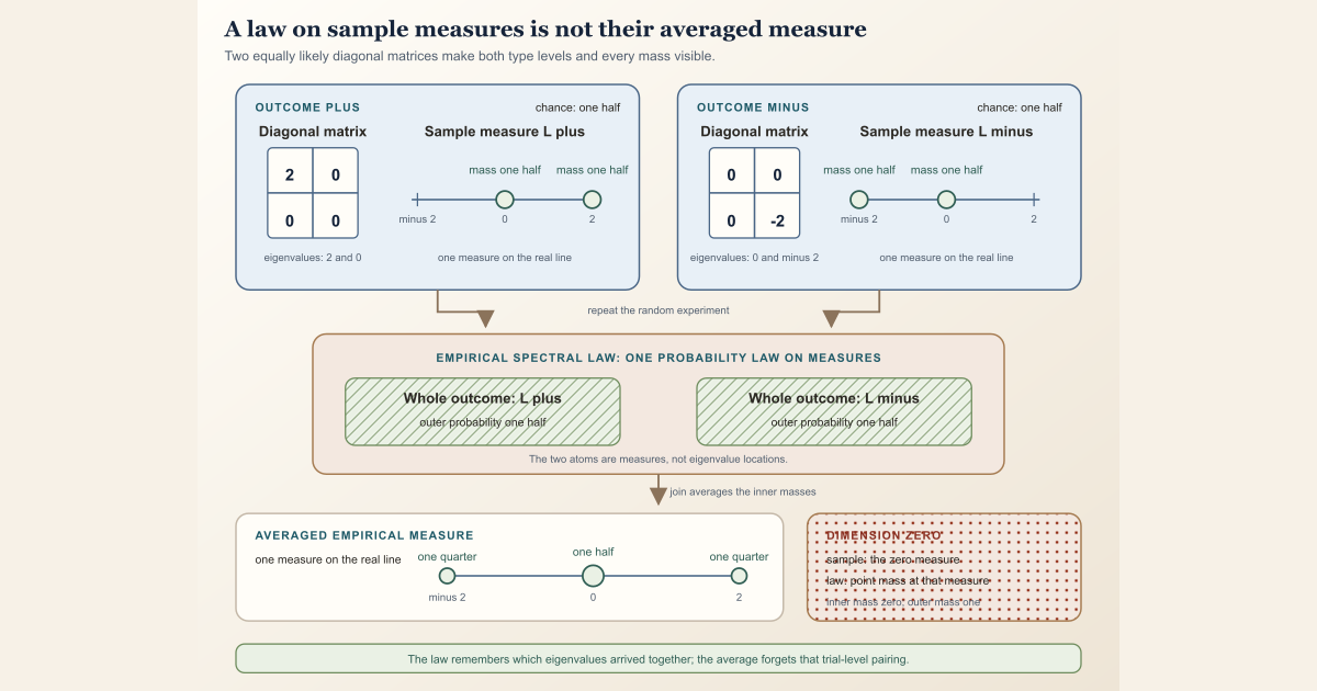
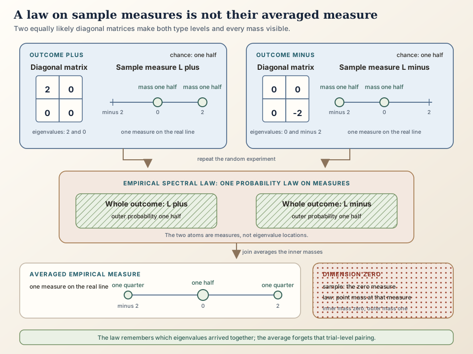
An empirical spectral law is the probability distribution, or law of a random matrix’s empirical spectral measure . One sampled matrix produces one measure on the real line. Repeating the experiment induces a probability distribution on a value space whose elements are whole measures.

That sentence contains three levels:

a sampled Hermitian matrix \(H\);
its empirical spectral measure \(L_H\), one measure on \(\mathbb R\); and
the law \(\mathcal Q\) of the measure-valued random variable \(H\mapsto L_H\).

An averaged empirical measure is a fourth object. It is one measure on \(\mathbb R\), not another name for \(\mathcal Q\).

Start with two equally likely matrices

Let the finite sample space be

\[ \Omega=\{+,-\}, \qquad \mathbb P(\{+\})=\mathbb P(\{-\})=\frac12. \]

Every subset of this two-point space is declared measurable. Define a matrix-valued random variable by

\[ H(+)= \begin{bmatrix} 2&0\\ 0&0 \end{bmatrix}, \qquad H(-)= \begin{bmatrix} 0&0\\ 0&-2 \end{bmatrix}. \]

Both matrices are diagonal and Hermitian, so their eigenvalues can be read directly from the diagonal:

Outcome	Eigenvalues, with multiplicity	Empirical spectral measure
\(+\)	\(2,0\)	\(L_+=\frac12\delta_2+\frac12\delta_0\)
\(-\)	\(0,-2\)	\(L_-=\frac12\delta_0+\frac12\delta_{-2}\)

Here \(\delta_x\) is the Dirac measure that puts one unit of mass at the real number \(x\). Because each matrix has two eigenvalues, each occurrence receives mass \(1/2\).

The two sample measures are different. For example,

\[ L_+(\{2\})=\frac12, \qquad L_-(\{2\})=0. \]

The law has whole measures as its atoms

Define the measure-valued map

\[ L:\Omega\to\operatorname{Measure}(\mathbb R), \qquad L(\omega)=L_{H(\omega)}. \]

Its probability law is the pushforward of \(\mathbb P\):

\[ \mathcal Q=L_*\mathbb P =\frac12\delta_{L_+}+\frac12\delta_{L_-}. \]

The two atoms of \(\mathcal Q\) are \(L_+\) and \(L_-\). They are measures. They are not the eigenvalue locations \(2,0,-2\). Sampling from \(\mathcal Q\) returns an entire spectral measure:

with outer probability \(1/2\), the result is \(L_+\);
with outer probability \(1/2\), the result is \(L_-\).

The nested type is therefore

\[ \mathcal Q:\operatorname{Measure} \bigl(\operatorname{Measure}(\mathbb R)\bigr). \]

Averaging gives a different object

Now average the inner measures:

\[ \begin{aligned} \overline L &=\frac12L_+ + \frac12L_-\\ &=\frac14\delta_2+\frac12\delta_0+\frac14\delta_{-2}. \end{aligned} \]

The coefficient at \(2\) is

\[ \frac12\text{ chance of outcome }+ \;\times\; \frac12\text{ spectral mass at }2 =\frac14. \]

The same calculation gives mass \(1/4\) at \(-2\). Both trials place half of their spectral mass at \(0\), so the average places mass \(1/2\) there.

The law and the average answer different questions:

Object	Type	What one sample returns	Information retained
\(\mathcal Q\)	measure on measures	either \(L_+\) or \(L_-\)	which eigenvalues appeared together in one trial
\(\overline L\)	measure on \(\mathbb R\)	one real location if sampled	only the averaged mass at each location

The distinction is not cosmetic. Let

\[ \mathcal Q_{\mathrm{det}}=\delta_{\overline L}. \]

This deterministic law always returns the single measure \(\overline L\). Its average is still \(\overline L\), but \(\mathcal Q_{\mathrm{det}}\ne\mathcal Q\). Thus two different laws on measures can have the same averaged measure. Averaging has discarded the sample-to-sample variation.

Two equally likely diagonal matrices have spectra two and zero, or zero and minus two. Their sample empirical measures each place mass one half on two locations. The empirical spectral law has those two whole measures as atoms, each with outer probability one half. The averaged empirical measure instead places masses one quarter, one half, and one quarter at minus two, zero, and two. — FigureFinding: the empirical spectral law retains the two measure-valued atoms \(L_+\) and \(L_-\), each with probability \(1/2\). The averaged measure combines their inner masses into \(1/4\) at \(-2\), \(1/2\) at \(0\), and \(1/4\) at \(2\), thereby discarding which nonzero eigenvalue occurred alongside zero. At dimension zero, the sample outcome is the zero measure, while the outer law is still a probability law concentrated at that outcome. The plate is a finite toy model, not a Gaussian unitary ensemble calculation or an asymptotic claim.

The general pushforward definition

Fix a dimension \(n\). Let \(\mathcal H_n\) be the finite-dimensional space of Hermitian matrices, let \(\mathbb P_n\) be a probability measure on that space, and let

\[ L_n:\mathcal H_n\to\operatorname{Measure}(\mathbb R) \]

send each matrix to its empirical spectral measure. If \(L_n\) is a measurable function , its empirical spectral law is

\[ \mathcal Q_n=(L_n)_*\mathbb P_n. \]

For a measurable collection \(C\) of measures,

\[ \mathcal Q_n(C) {} = \mathbb P_n\bigl(\{H\in\mathcal H_n:L_H\in C\}\bigr). \]

The pushforward rule says: to ask whether the random empirical measure lands in \(C\), pull \(C\) back to the matrix sample space and measure that event there.

Measurability is not a decorative side condition. The space Measure ℝ carries Mathlib’s Giry measurable structure, generated by evaluation of measures on measurable subsets of \(\mathbb R\). The project proves RandomMatrix.measurable_empiricalSpectralMeasure before using the map as a genuine probability observable. In the two-point example above, measurability was automatic only because every subset of the finite sample space was declared measurable.

In Lean: push the matrix law through the observable

One idea, three languages Read across, then read the syntax map

A human says

Sample an intrinsic finite Gaussian unitary ensemble matrix, form its empirical spectral measure, and take the probability law of that measure-valued output.

On paper

\(\mathcal Q_n=(L_n)_*\mathbb P_n\).

In Lean

GUE.empiricalSpectralLaw n = (GUE.intrinsicLaw n).map RandomMatrix.empiricalSpectralMeasure

Syntax map

GUE.intrinsicLaw n is the input Measure (RandomMatrix.HermitianEuclidean n).
RandomMatrix.empiricalSpectralMeasure is the observable from one intrinsic Hermitian matrix to one Measure ℝ.
.map is Mathlib’s pushforward operation. It transports the input probability mass through that observable.
The result has type Measure (Measure ℝ). The first Measure is the random law; each point in its carrier is an inner spectral measure.
The equality unfolds the project’s definition. The probability interpretation additionally uses RandomMatrix.measurable_empiricalSpectralMeasure.

The averaged empirical measure uses a different operation.

One idea, three languages Read across, then read the syntax map

A human says

Average the measure-valued outcomes of the empirical spectral law into one measure on the real line.

On paper

\(\overline L_n=\operatorname{join}(\mathcal Q_n)\).

In Lean

GUE.meanEmpiricalSpectralMeasure n = (GUE.empiricalSpectralLaw n).join

Syntax map

.join flattens one Measure (Measure ℝ) into one Measure ℝ by integrating the inner measures.
The left side and right side both have type Measure ℝ.
This operation removes the outer trial level. It is not another pushforward law.
This equality also unfolds a definition. It does not by itself justify exchanging an unbounded spectral-moment integral with the averaging step.

Exact checked source

Inside NonlinearDynamics.Random.GUE, with RandomMatrix opened, the pinned project contains these exact definitions:

noncomputable def empiricalSpectralLaw (n : ℕ) : Measure (Measure ℝ) :=
  (intrinsicLaw n).map empiricalSpectralMeasure

noncomputable def meanEmpiricalSpectralMeasure (n : ℕ) : Measure ℝ :=
  (empiricalSpectralLaw n).join

The imported continuity module supplies the measurable-observable gate inside NonlinearDynamics.Random.RandomMatrix:

theorem measurable_empiricalSpectralMeasure {n : ℕ} :
    Measurable (@empiricalSpectralMeasure n) :=
  measurable_empiricalSpectralMeasure_of_measurable_eigenvalues
    measurable_orderedHermitianEigenvalues_apply

The dimension-zero theorem is also explicit:

@[simp] theorem empiricalSpectralLaw_zero :
    empiricalSpectralLaw 0 = Measure.dirac (0 : Measure ℝ) := by
  rw [empiricalSpectralLaw, intrinsicLaw_zero]
  rw [Measure.map_dirac' measurable_empiricalSpectralMeasure]
  simp

The type annotation (0 : Measure ℝ) says that the point inside the outer Dirac law is the zero measure, not the real number zero. The proof maps the deterministic zero-dimensional matrix law through the measurable sample observable.

Try the toy type separation locally with Lean and Std

This worksheet encodes the two-outcome calculation without importing Mathlib. Each field stores mass in quarter-units: 4 means total mass one, 2 means one half, and 1 means one quarter. A list of two entries represents the two equally likely possible measure-valued outcomes.

Save it as EmpiricalSpectralLawTutorial.lean outside the project’s formalization/ directory:

import Std

inductive Outcome where
  | plus
  | minus
  deriving DecidableEq, Repr

structure SpectralMass where
  atNegTwo : Nat
  atZero : Nat
  atPosTwo : Nat
  deriving DecidableEq, Repr

def sampleMeasure : Outcome → SpectralMass
  | .plus =>
      { atNegTwo := 0, atZero := 2, atPosTwo := 2 }
  | .minus =>
      { atNegTwo := 2, atZero := 2, atPosTwo := 0 }

def empiricalSpectralLaw : List SpectralMass :=
  [sampleMeasure .plus, sampleMeasure .minus]

def averagedMeasure : SpectralMass :=
  { atNegTwo := 1, atZero := 2, atPosTwo := 1 }

def lawAtomCount (μ : SpectralMass) : Nat :=
  (empiricalSpectralLaw.filter fun ν => decide (ν = μ)).length

#eval sampleMeasure .plus
#eval sampleMeasure .minus
#eval empiricalSpectralLaw
#eval averagedMeasure

example : lawAtomCount (sampleMeasure .plus) = 1 := by decide
example : lawAtomCount (sampleMeasure .minus) = 1 := by decide
example : lawAtomCount averagedMeasure = 0 := by decide
example : averagedMeasure.atZero = 2 := by decide
example : empiricalSpectralLaw ≠ [averagedMeasure, averagedMeasure] := by decide

Run it with the repository’s pinned compiler:

elan run leanprover/lean4:v4.32.0 lean EmpiricalSpectralLawTutorial.lean

The first two outputs are the two sample empirical measures. The list output is the law’s two-point support, while averagedMeasure is one different record. The third proof shows that the average is not even a possible trial in this example. This is a finite type-and-arithmetic tutorial, not a construction of Mathlib measures, eigenvalues, measurability, or the Gaussian unitary ensemble.

Try the exact project interfaces

Try it in the repository NonlinearDynamics/Random/RandomMatrices/GaussianUnitaryEnsembleSpectrum.lean

The authoritative checked source is formalization/NonlinearDynamics/Random/RandomMatrices/GaussianUnitaryEnsembleSpectrum.lean. On a clone with the repository’s pinned dependencies installed, a human can type this import and declaration audit into a scratch file:

import NonlinearDynamics.Random.RandomMatrices.GaussianUnitaryEnsembleSpectrum

open MeasureTheory
open NonlinearDynamics.Random

#check RandomMatrix.empiricalSpectralMeasure
#check RandomMatrix.measurable_empiricalSpectralMeasure
#check GUE.empiricalSpectralLaw
#check GUE.instIsProbabilityMeasureEmpiricalSpectralLaw
#check GUE.empiricalSpectralLawProbability
#check GUE.empiricalSpectralProbabilityLaw
#check GUE.map_empiricalSpectralProbabilityLaw_coe
#check GUE.empiricalSpectralLaw_eq_map_matrixLaw_ambient
#check GUE.empiricalSpectralLaw_zero
#check GUE.meanEmpiricalSpectralMeasure
#check GUE.meanEmpiricalSpectralMeasure_zero
#check GUE.meanEmpiricalSpectralMeasure_succ_isProbability
#check Measure.join

The first two declarations are the sample observable and its measurability gate. The next group exposes the raw law and its two probability wrappers. The ambient transport theorem, zero-dimensional law, joined mean, and positive-dimensional mass theorem make the type and boundary policies inspectable by name. The generated full-project command below checks the complete project module; it does not run the small Std worksheet.

Full project check, from the repository root

cd formalization
lake env lean -DwarningAsError=true NonlinearDynamics/Random/RandomMatrices/GaussianUnitaryEnsembleSpectrum.lean

Resource note: this exact file uses the repository's pinned Lean and Mathlib dependencies. Initial project setup can require substantial disk space and build time. For a lightweight first step on macOS or Linux, use the page's standalone Lean-core or Std tutorial.

Four project objects that must remain separate

Project object	Lean type	What varies?	Total mass
Matrix sample \(H\)	`HermitianEuclidean n`	matrix entries	not a measure
Sample measure \(L_H\)	`Measure ℝ`	eigenvalue locations of one matrix	one for \(n\gt0\); zero for \(n=0\)
Law \(\mathcal Q_n\)	`Measure (Measure ℝ)`	which whole sample measure occurred	one in every dimension
Mean measure \(\overline L_n\)	`Measure ℝ`	no trial remains after joining	one for \(n\gt0\); zero for \(n=0\)

The law and mean can both be used to answer spectral questions, but the questions have different types. A set accepted by \(\mathcal Q_n\) is a collection of measures. A set accepted by \(\overline L_n\) is a collection of real eigenvalue locations.

Raw measures and bundled probability measures

The raw sample observable deliberately returns Measure ℝ in every dimension. In positive dimension, the project proves each sample measure has mass one and packages it as

RandomMatrix.empiricalSpectralProbability (n : ℕ) :
    HermitianEuclidean (n + 1) → ProbabilityMeasure ℝ

Pushing the intrinsic matrix law through this positive-dimensional observable gives

GUE.empiricalSpectralProbabilityLaw (n : ℕ) :
    ProbabilityMeasure (ProbabilityMeasure ℝ)

The parameter \(n\) here corresponds to matrix dimension \(n+1\). The successor form puts positivity in the type.

The raw outer law also has total mass one in every dimension, so it can be packaged as

GUE.empiricalSpectralLawProbability (n : ℕ) :
    ProbabilityMeasure (Measure ℝ)

These similarly named objects certify different facts:

empiricalSpectralLawProbability n says the outer law is a probability measure; its outcomes remain raw Measure ℝ values.
empiricalSpectralProbabilityLaw n exists in positive matrix dimension and bundles each inner outcome as a ProbabilityMeasure ℝ.

The theorem GUE.map_empiricalSpectralProbabilityLaw_coe proves that forgetting the positive-dimensional inner wrapper recovers GUE.empiricalSpectralLaw (n + 1). Wrapping carries a mass-one proof; it does not move spectral mass.

Dimension zero: inner mass zero, outer mass one

The empty spectrum forces the type distinction into the open. The sample empirical measure is defined by

\[ L_H=(n:\mathbb R_{\ge0}^{\infty})^{-1}N_H, \]

where \(N_H\) is the spectral counting measure. At \(n=0\), the counting measure is zero because there are no eigenvalue indices. The extended nonnegative inverse of zero is infinity, but the scalar action on the zero measure still yields the zero measure:

\[ L_H=0. \]

This inner zero measure has total mass zero, so it cannot be bundled as a ProbabilityMeasure ℝ. The zero-dimensional intrinsic matrix law, however, is concentrated at the unique empty matrix. Pushing it forward gives

\[ \mathcal Q_0=\delta_{0:\operatorname{Measure}(\mathbb R)}. \]

The outer Dirac law has total mass one. Its only outcome is the inner zero measure. Joining that law gives

\[ \overline L_0=0. \]

Thus the raw empirical spectral law and its outer probability wrapper make sense in every dimension. The probability-measure-valued sample law is exposed only for positive dimensions.

The mean is a Giry join

Mathlib’s Measure.join integrates inner measures set by set. For a measurable set \(B\subseteq\mathbb R\), the intended reading is

\[ \overline L_n(B) {} = \int_{\operatorname{Measure}(\mathbb R)} \mu(B)\,\mathrm d\mathcal Q_n(\mu). \]

The project proves GUE.meanEmpiricalSpectralMeasure_succ_isProbability: in positive dimension, the joined mean has mass one. At dimension zero, the checked mean is the zero measure.

Joining measures is not automatically a theorem about every unbounded integrand. In particular, the checked module does not prove

\[ \int_{\mathbb R}(x:\mathbb C)^k\,\mathrm d\overline L_n(x) \stackrel{?}{=} \int_{\mathcal H_n} \left(\int_{\mathbb R}(x:\mathbb C)^k\,\mathrm dL_H(x)\right) \mathrm d\mathbb P_n(H). \]

Such an interchange needs the appropriate measurability and integrability theorem. The page keeps it separate from the definition of the mean measure.

What the checked module additionally proves about moments

For one Hermitian matrix sample, the \(k\)-th complex empirical spectral moment is

\[ m_k(H)=\int_{\mathbb R}(x:\mathbb C)^k\,\mathrm dL_H(x). \]

The first two checked sample identities are

\[ m_1(H)= \left(\frac1n:\mathbb C\right)\operatorname{Tr}(H), \qquad m_2(H)= \left(\frac1n:\mathbb C\right)\operatorname{Tr}(H^2). \]

They hold under the project’s totalized dimension-zero convention. For the project’s Wigner-scaled finite Gaussian unitary ensemble (GUE),

\[ \mathbb E[m_1(H)]=0, \qquad \mathbb E[m_2(H)] {} = \left(\frac1n:\mathbb C\right)n. \]

The second expectation is zero for \(n=0\) and one for \(n\gt0\). These are expectations of sample-moment observables under the matrix law. They are not moments of the joined mean measure unless the missing interchange theorem is separately supplied.

Intrinsic and ambient matrix presentations agree

The finite GUE law has two compatible carriers:

GUE.intrinsicLaw n lives on intrinsic Hermitian matrices;
GUE.matrixLaw n lives on all complex square matrices and gives the Hermitian locus full mass.

The ambient empirical-spectral observable sends a Hermitian matrix to its intrinsic empirical measure and sends a non-Hermitian input to zero. The project proves

\[ \mathcal Q_n {} = (\operatorname{ambientEmpiricalSpectralMeasure})_* \operatorname{matrixLaw}_n. \]

The non-Hermitian fallback is irrelevant almost everywhere under finite GUE because the ambient law is supported on Hermitian matrices. This is a pushforward identity, not a spectral theory for arbitrary non-Hermitian matrices.

Boundaries that prevent common mistakes

Tempting claim	Correct statement
“An empirical spectral law is the eigenvalue histogram of one matrix.”	One histogram-like empirical measure is a sample; the law describes how that whole measure varies across trials.
“The law and the averaged empirical measure are equal.”	They live in different spaces: `Measure (Measure ℝ)` versus `Measure ℝ`.
“Knowing the average determines the law.”	The toy \(\mathcal Q\) and deterministic \(\delta_{\overline L}\) have the same average but different trial variation.
“Matching mean spectral mass proves matching random spectra.”	Different joint patterns of eigenvalues can average to the same measure.
“A map to measures automatically has a law.”	Its pushforward interpretation requires a measurable, or at least appropriately almost-everywhere measurable, observable.
“Every sample empirical measure is a probability measure.”	It has mass one in positive dimension; the dimension-zero sample measure is zero.
“The zero-dimensional law has mass zero.”	Its unique inner outcome has mass zero, but the outer Dirac law has mass one.
“The moment of the mean is already the expected sample moment.”	That interchange needs its own checked measurability and integrability result.

Exercises

Verify all three coefficients in \(\overline L=\frac14\delta_2+\frac12\delta_0+ \frac14\delta_{-2}\).
Compute the first moment of \(L_+\), \(L_-\), and \(\overline L\). Which information disappears after averaging?
Explain why \(\mathcal Q\) and \(\delta_{\overline L}\) have the same mean but are different probability laws on measures.
State the domain and codomain of the sample map \(L_n\), then identify the domain and codomain of the resulting pushforward law.
Explain why the zero measure can be an outcome of a probability law without itself being a probability measure.
Name the theorem needed before treating an expected sample moment as a moment of the joined mean measure.

Where to continue

The empirical spectral measure entry develops the one-sample object and its multiplicity convention. Pushforward measure explains the law-forming operation independently of random matrices.

Finite GUE Empirical Spectral Laws and Normalized Moments builds the complete finite-GUE law, probability packaging, Giry join, and moment transport from the checked declarations. Hermitian Spectral Perturbation, Continuity, and Measurability proves the measurability gate that makes the law available.

References

Project source. GaussianUnitaryEnsembleSpectrum.lean, the pinned definitions and theorems for the empirical spectral law, its probability packaging, its dimension-zero branch, the joined mean measure, and the first two finite-GUE sample-moment expectations.

Mathlib contributors. The Giry measurable structure on measures, Mathlib 4 documentation. This official page defines the measurable structure on Measure α and documents measurable_map, join, join_apply, and measurable_join.

Mathlib contributors. Probability measures, Mathlib 4 documentation. This official page defines ProbabilityMeasure α, its coercion to raw measures, measurable pushforward, and probability status under joining.

Michèle Giry. A Categorical Approach to Probability Theory, in Categorical Aspects of Topology and Analysis, Lecture Notes in Mathematics 915, Springer, 1982, pp. 68-85. This primary source introduced the measure-valued monadic framework that motivates the name Giry; exact claims here use Mathlib’s checked implementation.

Greg W. Anderson, Alice Guionnet, and Ofer Zeitouni. An Introduction to Random Matrices, Cambridge University Press, 2010. Chapters 2 and 3 treat empirical eigenvalue measures, Wigner scaling, Gaussian ensembles, and their asymptotic role. This page uses only the finite empirical-measure convention and states the project’s normalization separately.

The exact upstream Lean source audited for this entry is Mathlib commit 81a5d257, the revision pinned by formalization/lake-manifest.json.