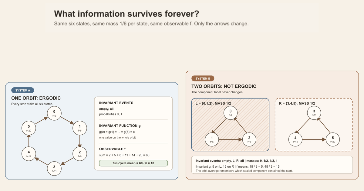
Start with six equally likely states
Let the space of possible states be
\[ \Omega=\{0,1,2,3,4,5\}. \]Give every state probability \(1/6\). Thus an event \(S\subseteq\Omega\) has probability
\[ \mu(S)=\frac{|S|}{6}, \]where \(|S|\) is the number of states in \(S\). Every subset is measurable in this finite example.
Put the following real-valued observable on the states:
\[ \begin{array}{c|rrrrrr} x&0&1&2&3&4&5\\ \hline f(x)&2&5&8&11&14&20 \end{array} \]An observable is a quantity read from the current state. Here it is the function \(f:\Omega\to\mathbb R\).
We will keep the same states, probabilities, and observable while changing only the time-one map.
System A: one orbit visits all six states
Define
\[ T_{\mathrm{one}}: 0\mapsto1\mapsto2\mapsto3\mapsto4\mapsto5\mapsto0. \]This permutation preserves the uniform probability: the preimage of an event has exactly as many points as the event itself. Starting at any state, six steps visit every state exactly once. The six-step sum is
\[ 2+5+8+11+14+20=60, \]so the six-step average is
\[ \frac{60}{6}=10. \]Now ask which events are unchanged by one step. An event \(S\) is strictly invariant when
\[ T_{\mathrm{one}}^{-1}(S)=S. \]The symbol \(T^{-1}(S)\) means preimage, not an inverse function:
\[ x\in T^{-1}(S) \quad\Longleftrightarrow\quad T(x)\in S. \]If a strictly invariant event contains one state, moving forward around the cycle shows that it contains all six. Therefore the complete invariant-event list is
\[ \varnothing,\qquad \Omega, \]with probabilities \(0\) and \(1\). There is no invariant region holding a proper positive fraction of the probability. The system is ergodic.
System B: two sealed three-state orbits
Define instead
\[ \begin{aligned} T_{\mathrm{split}}:\;&0\mapsto1\mapsto2\mapsto0,\\ &3\mapsto4\mapsto5\mapsto3. \end{aligned} \]This map is also a permutation, so it preserves exactly the same uniform probability. But the event
\[ L=\{0,1,2\} \]is now strictly invariant:
\[ T_{\mathrm{split}}^{-1}(L)=L, \qquad \mu(L)=\frac36=\frac12. \]Its complement \(R=\{3,4,5\}\) is also invariant and has probability \(1/2\). The complete invariant-event list is
\[ \varnothing,\qquad L,\qquad R,\qquad\Omega, \]with probabilities \(0,1/2,1/2,1\). The invariant events \(L\) and \(R\), each of probability \(1/2\), violate the null-or-conull criterion. Therefore this system is not ergodic.
The observable also exposes the split. Its average around the left orbit is
\[ \frac{2+5+8}{3}=5, \]while its average around the right orbit is
\[ \frac{11+14+20}{3}=15. \]Starting anywhere in \(L\), every complete three-step block averages to \(5\). Starting anywhere in \(R\), every complete three-step block averages to \(15\). The dynamics retain one bit of durable information: which component did the orbit start in?
What the example teaches
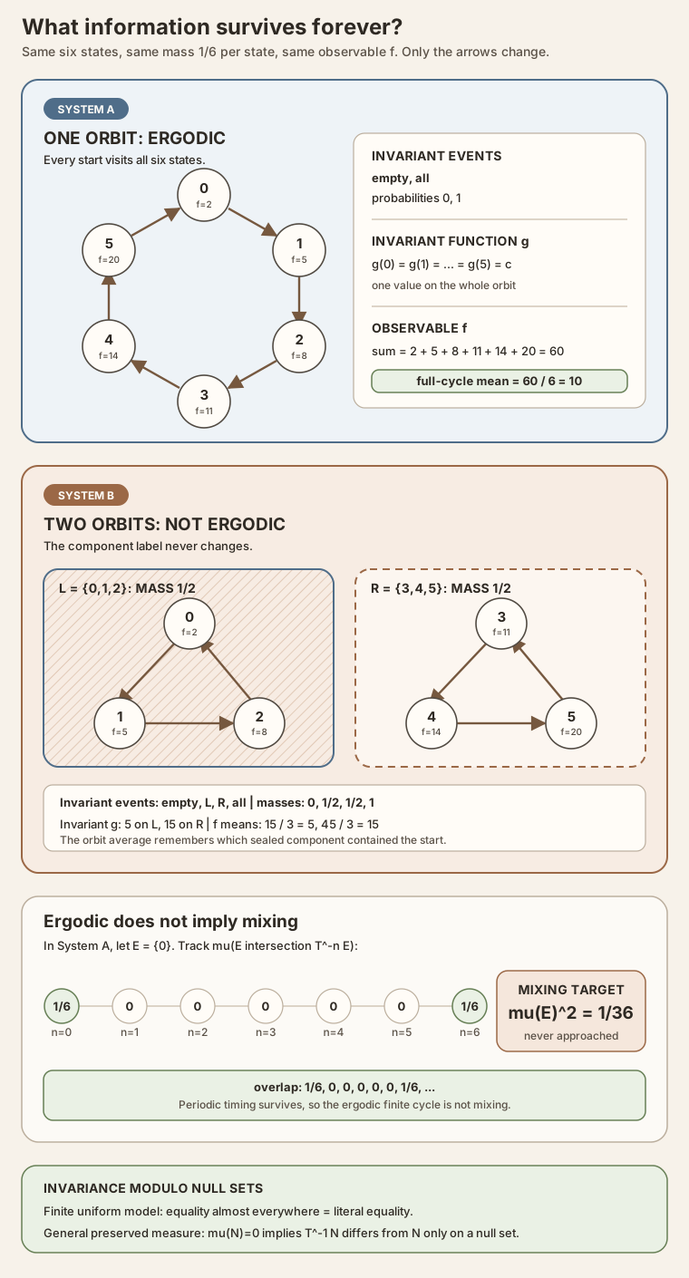
Ergodicity is a statement about invariant information, not about whether an orbit moves.
- Both examples move every state and preserve probability.
- The one-cycle system eventually carries every start through the same six states.
- The split system never carries a point from \(L\) to \(R\) or from \(R\) to \(L\).
- The component label is therefore an invariant distinction with probability \(1/2\) on each side.
This page’s six-state calculation complements Ergodic probability base . That entry separates probability normalization, measure preservation, and ergodic rigidity. Here the focus is the exact information that survives, its function-valued form, its effect on time averages, and its sharp separation from mixing.
The general definition
Let \((\Omega,\mathcal B)\) be a measurable space and let \(\mu\) be a measure on it:
- \(\Omega\) is the state space;
- \(\mathcal B\) is the collection of measurable events;
- \(\mu\) is a measure assigning sizes to those events; and
- \(T:\Omega\to\Omega\) is the time-one map.
The map is measure preserving when it is measurable and
\[ \mu(T^{-1}S)=\mu(S) \]for every measurable event \(S\).
The system is ergodic when it is measure preserving and every measurable strictly invariant event is null or conull:
\[ T^{-1}S=S \quad\Longrightarrow\quad \mu(S)=0 \ \text{or}\ \mu(S^{\mathsf c})=0. \]Here \(S^{\mathsf c}=\Omega\setminus S\) is the complement of \(S\). A null set has measure zero. A conull event has a null complement, so it contains almost all measured states. On a probability space , where \(\mu(\Omega)=1\), the conclusion becomes
\[ \mu(S)=0 \quad\text{or}\quad \mu(S)=1. \]The number \(1\) comes from probability normalization, not from ergodicity alone. If the total mass were \(6\), a conull event would have mass \(6\).
Event form and function form
There are two closely related ways to detect invariant information.
Invariant events
An invariant event asks a yes-or-no question whose answer never changes along an orbit:
\[ \mathbf 1_S(Tx)=\mathbf 1_S(x). \]The indicator \(\mathbf 1_S\) equals \(1\) on \(S\) and \(0\) outside it. In the split example, \(\mathbf 1_L\) records which of the two orbit components contains \(x\).
Invariant functions
A measurable function \(g:\Omega\to\mathbb R\) is invariant when
\[ g\circ T=g, \qquad\text{equivalently}\qquad g(Tx)=g(x) \]for every \(x\). Such a function assigns one fixed value along each orbit.
For the one six-cycle, invariance forces the chain
\[ g(0)=g(1)=g(2)=g(3)=g(4)=g(5). \]For the split map, the function
\[ g(x)= \begin{cases} 5,&x\in L,\\ 15,&x\in R \end{cases} \]is invariant and nonconstant. It stores the same component information as the event \(L\).
In a general ergodic system, a suitably measurable invariant function is constant almost everywhere . “Almost everywhere” means that the equality may fail on a null set. It does not mean pointwise equality at every state.
Strict invariance versus invariance modulo null sets
Three set statements must be kept separate:
- Strict invariance: \(T^{-1}S=S\) as literal sets.
- Almost invariance: \(T^{-1}S\) and \(S\) differ only on a null set.
- Trivial modulo null sets: \(S\) differs from \(\varnothing\) or \(\Omega\) only on a null set.
The symmetric difference
\[ \begin{aligned} A\mathbin{\triangle}B &=(A\setminus B)\cup(B\setminus A). \end{aligned} \]contains the points on which membership in \(A\) and \(B\) disagrees. Almost invariance can therefore be written
\[ \mu\!\left(T^{-1}S\mathbin{\triangle}S\right)=0. \]Equivalently, Mathlib writes equality of the sets almost everywhere:
\[ T^{-1}S =_{\mu\text{-a.e.}} S. \]In the finite uniform six-state model, every nonempty event has positive probability. The only null event is \(\varnothing\), so equality modulo null sets is exactly ordinary equality. That is why the finite list of invariant events can be computed without qualifications.
General spaces can have nonempty null sets. Suppose \(N\) is null and \(T\) preserves \(\mu\). Then \(T^{-1}N\) is also null, and
\[ T^{-1}N\mathbin{\triangle}N \subseteq T^{-1}N\cup N \]is null. Thus \(N\) is almost invariant even if \(T^{-1}N\ne N\) pointwise. This is not a violation of ergodicity: \(N\) already represents the same measured event as \(\varnothing\).
Mathlib exposes this distinction deliberately:
PreErgodicis defined using strict invariance of a measurable set;QuasiErgodic.ae_empty_or_univ₀accepts a null-measurable, almost invariant set; and- every
Ergodicmap yields the neededQuasiErgodicinterface throughhT.quasiErgodic.
The subscript zero in these Mathlib theorem names is part of the library identifier; it is not the probability value zero.
Ergodic does not mean mixing
Ergodicity rules out invariant distinctions. Strong mixing asks for a different, stronger property: widely separated observations should lose their correlation. On a probability space, one standard form is
\[ \mu\!\left(E\cap T^{-n}F\right) \longrightarrow \mu(E)\mu(F) \qquad(n\to\infty) \]for every pair of measurable events \(E,F\).
Return to the ergodic six-cycle and take
\[ E=F=\{0\}. \]Because the orbit returns to \(0\) exactly at multiples of six,
\[ \mu\!\left(E\cap T_{\mathrm{one}}^{-n}E\right) {} = \begin{cases} 1/6,&6\mid n,\\ 0,&6\nmid n. \end{cases} \]Here \(6\mid n\) means that \(6\) divides \(n\). The proposed mixing target is
\[ \mu(E)\mu(E)=\frac16\cdot\frac16=\frac1{36}. \]The overlap keeps cycling between \(1/6\) and \(0\), so it does not converge to \(1/36\). The map is ergodic but not mixing.
There is no paradox:
- ergodicity asks whether any event is unchanged forever;
- mixing asks whether long-lag overlaps approach a product; and
- a periodic orbit can have no proper invariant event while retaining perfect timing information.
The same system is a counterexample to the claim that ergodicity passes to every power. Since \(T_{\mathrm{one}}^6=\operatorname{id}\), every event is invariant under the sixth power, so \(T_{\mathrm{one}}^6\) is not ergodic.
Why time averages enter the story
For an observable \(f:\Omega\to\mathbb R\), the \(n\)-step Birkhoff average is
\[ \begin{aligned} A_n f(x) &=\frac1n\sum_{k=0}^{n-1}f(T^k x), \end{aligned} \qquad n\ge1. \]The notation \(T^k\) means apply \(T\) \(k\) times, as developed under orbit and iterate . In the one six-cycle, every block of six consecutive observations contains the same six values, so
\[ A_{6m}f(x)=10 \]for every start \(x\) and every positive integer \(m\).
In the split system,
\[ A_{3m}f(x)= \begin{cases} 5,&x\in L,\\ 15,&x\in R. \end{cases} \]The nonergodic limit is an invariant function: it is constant on each orbit component but not globally constant. Ergodicity is exactly the rigidity that collapses such invariant measurable targets to one almost-everywhere constant.
The project’s RMT-28 theorem applies this to the conditional expectation onto the invariant sigma algebra . Under an ergodic probability measure and integrability of \(f\), it identifies the almost-everywhere Birkhoff limit with the ordinary integral
\[ \int_\Omega f\,d\mu. \]Ergodicity by itself is not a convergence theorem. The Birkhoff theorem, measurability, integrability, and measure preservation still do real work.
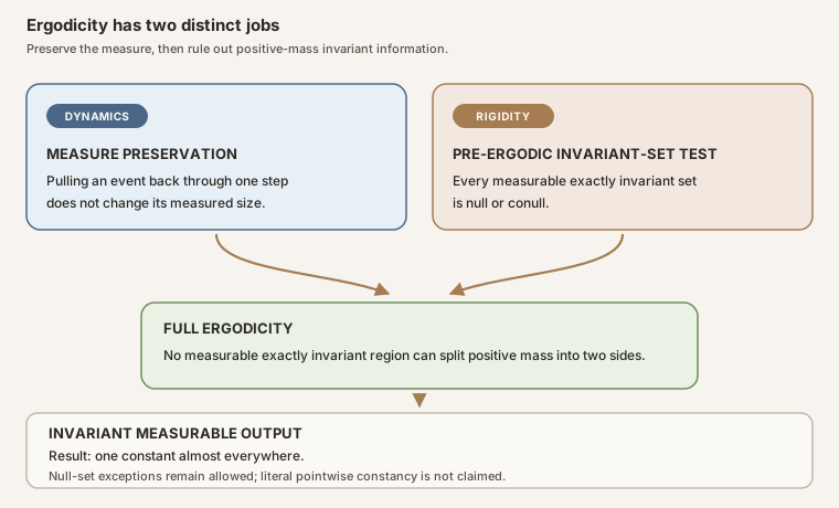
PreErgodic supplies the invariant-information rigidity used to collapse exact invariant measurable functions almost everywhere. Ergodic also contains measure preservation, which is needed when the project invokes the preceding Birkhoff convergence theorem. The diagram does not assert mixing, independence, pointwise constancy, or literal equality of the invariant sigma algebra with the bottom sigma algebra.In Lean: the same ideas in exact syntax
1. Say that an event is strictly invariant
T ⁻¹' S = SA human types:
#check T ⁻¹' S = S
The important symbols are:
Tis a function from states to states;⁻¹’is Lean’s set-preimage operator;Sis aSet Ω; and=is literal equality of sets, not equality modulo null sets.
No inverse function is being assumed. Lean reads
x ∈ T ⁻¹’ S as T x ∈ S.
2. Separate pre-ergodic rigidity from full ergodicity
hpre.ae_empty_or_univ hS hInvMathlib’s exact structures are:
structure PreErgodic (T : Ω → Ω) (μ : Measure Ω) : Prop where
  aeconst_set ⦃S : Set Ω⦄ :
    MeasurableSet S →
    T ⁻¹' S = S →
    EventuallyConst S (ae μ)

structure Ergodic (T : Ω → Ω) (μ : Measure Ω) : Prop extends
  MeasurePreserving T μ μ, PreErgodic T μ
The source uses implicit variables and a default measure argument; the excerpt above renames them for readability without changing the fields. A human asks for the interfaces and consequences with:
#check PreErgodic T μ
#check Ergodic T μ
#check hT.toPreErgodic
#check hT.toMeasurePreserving
#check hpre.ae_empty_or_univ hS hInv
#check hpre.measure_self_or_compl_eq_zero hS hInv
Token map:
hpre : PreErgodic T μis evidence of invariant-set rigidity;hT : Ergodic T μcontains both required fields;hS : MeasurableSet Ssays \(S\) belongs to the measurable space;hInv : T ⁻¹’ S = Sis strict invariance;ae μis the filter of statements true almost everywhere with respect to \(\mu\); andEventuallyConst S (ae μ)says membership in \(S\) is eventually one constant truth value in that filter.
3. Read the probability zero-one law
hpre.prob_eq_zero_or_one hS hInvWith [IsProbabilityMeasure μ] in scope, a human types:
#check hpre.prob_eq_zero_or_one hS hInv
- Square brackets tell Lean to find the probability-normalization instance.
prob_eq_zero_or_oneis a theorem in thePreErgodicnamespace.- Its result is a logical disjunction, written
∨. - The conclusion uses \(1\) because the measure is normalized to total mass one.
4. Move from strict to almost invariance
hT.quasiErgodic.ae_empty_or_univ₀ hNullMeas hAeInvA human types:
#check hT.quasiErgodic
#check hT.quasiErgodic.ae_empty_or_univ₀ hNullMeas hAeInv
hNullMeas : NullMeasurableSet S μpermits changing \(S\) on a null set to obtain a measurable representative.hAeInv : T ⁻¹’ S =ᵐ[μ] Sis almost-everywhere equality of the two set-valued membership predicates.=ᵐ[μ]is pronounced “equal almost everywhere with respect to \(\mu\).”hT.quasiErgodicconverts full ergodicity to the Mathlib interface whose theorem accepts almost invariance.
5. Collapse an invariant function
hT.ae_eq_const_of_ae_eq_comp_ae hg hGInvFor a real-valued \(g\), a human types:
#check hT.ae_eq_const_of_ae_eq_comp_ae hg hGInv
The inputs and output are:
hg : AEStronglyMeasurable g μis the almost-everywhere strong measurability certificate;hGInv : g ∘ T =ᵐ[μ] gsays composition with \(T\) does not change \(g\), except possibly on a null set;∘is function composition, so(g ∘ T) xreduces tog (T x); and- the theorem returns
∃ c, g =ᵐ[μ] Function.const Ω c.
This is the general version of “one value on the single six-cycle.” In the split example the nonconstant component-label function shows exactly why the ergodic hypothesis cannot be dropped.
6. Identify the ergodic Birkhoff limit
ae_tendsto_birkhoffAverage_integral_of_ergodic hT hfThe checked project theorem is:
theorem ae_tendsto_birkhoffAverage_integral_of_ergodic
    [IsProbabilityMeasure μ]
    (hT : Ergodic T μ) (hf : Integrable f μ) :
    ∀ᵐ ω ∂μ,
      Tendsto (fun n ↦ birkhoffAverage ℝ T f n ω) atTop
        (nhds (∫ x, f x ∂μ))
A human types:
#check ae_tendsto_birkhoffAverage_integral_of_ergodic hT hf
Read it left to right:
∀ᵐ ω ∂μmeans “for almost every \(\omega\) with respect to \(\mu\)”;birkhoffAverage ℝ T f n ωis the project’s totalized \(n\)-step time average;Tendsto … atTopmeans convergence as natural \(n\) becomes arbitrarily large;nhds ais the neighborhood filter around the proposed limit \(a\); and∫ x, f x ∂μis the integral, equal to the ordinary probabilityexpectation when \(\mu\) has total mass one.
This theorem uses full Ergodic. The preceding conditional-
expectation identification needs only PreErgodic, but the
Birkhoff convergence input needs measure preservation.
Exact source excerpts
Resource label: pinned Mathlib. The repository’s pinned
Mathlib/Dynamics/Ergodic/Ergodic.lean
contains:
structure PreErgodic (f : α → α) (μ : Measure α := by volume_tac) : Prop where
  aeconst_set ⦃s : Set α⦄ :
    MeasurableSet s → f ⁻¹' s = s → EventuallyConst s (ae μ)

structure Ergodic (f : α → α) (μ : Measure α := by volume_tac) : Prop extends
  MeasurePreserving f μ μ, PreErgodic f μ

theorem PreErgodic.prob_eq_zero_or_one
    [IsProbabilityMeasure μ]
    (hf : PreErgodic f μ) (hs : MeasurableSet s)
    (hs' : f ⁻¹' s = s) :
    μ s = 0 ∨ μ s = 1
The same file’s almost-invariant interface is:
theorem QuasiErgodic.ae_empty_or_univ₀
    (hf : QuasiErgodic f μ)
    (hsm : NullMeasurableSet s μ)
    (hs : f ⁻¹' s =ᵐ[μ] s) :
    s =ᵐ[μ] (∅ : Set α) ∨ s =ᵐ[μ] Set.univ
Resource label: pinned Mathlib.
Mathlib/Dynamics/Ergodic/Function.lean
contains:
theorem Ergodic.ae_eq_const_of_ae_eq_comp_ae
    {g : α → X} (h : Ergodic f μ)
    (hgm : AEStronglyMeasurable g μ)
    (hg_eq : g ∘ f =ᵐ[μ] g) :
    ∃ c, g =ᵐ[μ] Function.const α c
Resource label: checked project source.
ErgodicBirkhoffLimit.lean
uses the two projections separately:
filter_upwards
    [ae_tendsto_birkhoffAverage_condExp hT.toMeasurePreserving hf,
      condExp_invariants_ae_eq_integral_of_preErgodic
        (T := T) (f := f) hT.toPreErgodic hf]
    with ω hconv htarget
simpa only [htarget] using hconv
The first line supplies orbit-average convergence to an invariant conditional expectation. The second collapses that invariant target to the integral. The proof therefore records which half of ergodicity does which job.
Standalone tutorial
Standalone tutorial. This worksheet imports only
Std. It enumerates all \(64\) events, computes the invariant-event
lists for the two six-state maps, checks the component-label function, prints
six-step orbit sums, and prints the singleton-overlap pattern. It does not
formalize measure theory or prove the general ergodic theorem.
Save the following as ErgodicityFiniteScratch.lean:
import Std

def states : List Nat :=
  List.range 6

def oneCycle (x : Nat) : Nat :=
  (x + 1) % 6

def splitCycles (x : Nat) : Nat :=
  if x < 3 then
    (x + 1) % 3
  else
    3 + (x - 3 + 1) % 3

def subsets : List (List Nat) :=
  states.foldr
    (fun x acc => acc ++ acc.map (fun event => x :: event))
    [[]]

def preimage (T : Nat → Nat) (event : List Nat) : List Nat :=
  states.filter fun x => event.contains (T x)

def invariant (T : Nat → Nat) (event : List Nat) : Bool :=
  preimage T event == event

def invariantEvents (T : Nat → Nat) : List (List Nat) :=
  subsets.filter fun event => invariant T event

def observable : Nat → Int
  | 0 => 2
  | 1 => 5
  | 2 => 8
  | 3 => 11
  | 4 => 14
  | 5 => 20
  | _ => 0

def componentMean (x : Nat) : Int :=
  if x < 3 then 5 else 15

def invariantFunction (T : Nat → Nat) (g : Nat → Int) : Bool :=
  states.all fun x => decide (g (T x) = g x)

def iterate (T : Nat → Nat) : Nat → Nat → Nat
  | 0, x => x
  | n + 1, x => T (iterate T n x)

def orbitValues
    (T : Nat → Nat) (start steps : Nat) : List Int :=
  (List.range steps).map fun n => observable (iterate T n start)

def orbitSum
    (T : Nat → Nat) (start steps : Nat) : Int :=
  (orbitValues T start steps).foldl (fun total x => total + x) 0

def overlapCount
    (T : Nat → Nat) (event : List Nat) (n : Nat) : Nat :=
  ((preimage (fun x => iterate T n x) event).filter
    (fun x => event.contains x)).length

#eval invariantEvents oneCycle
#eval invariantEvents splitCycles
#eval invariantFunction oneCycle componentMean
#eval invariantFunction splitCycles componentMean
#eval states.map fun x =>
  (x, orbitValues oneCycle x 6, orbitSum oneCycle x 6)
#eval states.map fun x =>
  (x, orbitValues splitCycles x 6, orbitSum splitCycles x 6)
#eval (List.range 13).map fun n =>
  (n, overlapCount oneCycle [0] n)
Run it on an ordinary Mac or Linux machine with the pinned small toolchain:
source "$HOME/.elan/env"
elan run leanprover/lean4:v4.32.0 lean ErgodicityFiniteScratch.lean
This exact worksheet was executed successfully with the pinned Lean 4.32.0 compiler and printed:
[[], [0, 1, 2, 3, 4, 5]]
[[], [3, 4, 5], [0, 1, 2], [0, 1, 2, 3, 4, 5]]
false
true
[(0, [2, 5, 8, 11, 14, 20], 60),
 (1, [5, 8, 11, 14, 20, 2], 60),
 (2, [8, 11, 14, 20, 2, 5], 60),
 (3, [11, 14, 20, 2, 5, 8], 60),
 (4, [14, 20, 2, 5, 8, 11], 60),
 (5, [20, 2, 5, 8, 11, 14], 60)]
[(0, [2, 5, 8, 2, 5, 8], 30),
 (1, [5, 8, 2, 5, 8, 2], 30),
 (2, [8, 2, 5, 8, 2, 5], 30),
 (3, [11, 14, 20, 11, 14, 20], 90),
 (4, [14, 20, 11, 14, 20, 11], 90),
 (5, [20, 11, 14, 20, 11, 14], 90)]
[(0, 1), (1, 0), (2, 0), (3, 0), (4, 0), (5, 0), (6, 1), (7, 0), (8, 0), (9, 0), (10, 0), (11, 0), (12, 1)]
The first function check printed false; the second printed
true. Every one-cycle six-step sum is \(60\). Split starts
\(0,1,2\) have sum \(30\), and starts \(3,4,5\) have sum \(90\). The overlap
count for \(\{0\}\) is \(1\) at \(n=0,6,12\) and \(0\) at the other displayed
times.
Dividing those counts by six gives the overlap probabilities in the figure.
The worksheet is an executable audit of the finite arithmetic, not a proof
that an abstract measure-preserving system is ergodic. It imports only
Std and does not load the project or Mathlib.
Try it in the repository
Full project check. This uses the repository’s pinned Lean and Mathlib dependencies and may require substantial disk space and memory. Create a temporary project worksheet containing:
import NonlinearDynamics.Random.RandomCocycles.ErgodicBirkhoffLimit

open MeasureTheory Set Filter Function ProbabilityTheory
open NonlinearDynamics.Random.RandomCocycles
open scoped ENNReal Topology BigOperators

universe uΩ

variable {Ω : Type uΩ} [MeasurableSpace Ω]
variable {T : Ω → Ω} {μ : Measure Ω}
variable {S : Set Ω} {f g : Ω → ℝ}
variable [IsProbabilityMeasure μ]

variable (hpre : PreErgodic T μ)
variable (hT : Ergodic T μ)
variable (hS : MeasurableSet S)
variable (hInv : T ⁻¹' S = S)
variable (hNullMeas : NullMeasurableSet S μ)
variable (hAeInv : T ⁻¹' S =ᵐ[μ] S)
variable (hg : AEStronglyMeasurable g μ)
variable (hGInv : g ∘ T =ᵐ[μ] g)
variable (hf : Integrable f μ)

#check PreErgodic
#check Ergodic
#check QuasiErgodic
#check hT.toPreErgodic
#check hT.toMeasurePreserving
#check hT.quasiErgodic
#check hpre.ae_empty_or_univ hS hInv
#check hpre.measure_self_or_compl_eq_zero hS hInv
#check hpre.prob_eq_zero_or_one hS hInv
#check hT.quasiErgodic.ae_empty_or_univ₀ hNullMeas hAeInv
#check hT.ae_eq_const_of_ae_eq_comp_ae hg hGInv
#check condExp_invariants_comp
#check condExp_invariants_ae_eq_integral_of_preErgodic
#check ae_tendsto_birkhoffAverage_integral_of_ergodic hT hf
Each #check asks the pinned elaborator for the declaration’s exact
type. The current project leaf is checked with:
cd formalization
lake env lean NonlinearDynamics/Random/RandomCocycles/ErgodicBirkhoffLimit.lean
This full project check uses the repository’s pinned Lean and Mathlib dependencies and may require substantial disk space and memory.
cd formalization
lake env lean -DwarningAsError=true NonlinearDynamics/Random/RandomCocycles/ErgodicBirkhoffLimit.lean
Resource note: this exact file uses the repository's
pinned Lean and Mathlib dependencies. Initial project setup can require
substantial disk space and build time. For a lightweight first step on
macOS or Linux, use the page's standalone Lean-core or Std
tutorial.
Boundary cases and common traps
Identity dynamics
If \(T=\operatorname{id}\), every event is strictly invariant. On two atoms with positive mass, either singleton is a positive-mass invariant event with a positive-mass complement. The system is not pre-ergodic and therefore not ergodic. A function that assigns different values to the atoms is invariant and nonconstant.
A Dirac measure
A Dirac measure places all mass at one point. Every event is then null or
conull, so PreErgodic T μ can hold even when \(T\) does not
preserve \(\mu\). The project contains a checked instance of this boundary
model. That model is a counterexample to any implication from pre-ergodicity
alone to measure preservation.
The zero measure
Under Mathlib’s definition, a measurable map is ergodic with respect to the zero measure. Every event is both null and conull, and every almost-everywhere statement is vacuous. Consequently,
\[ \text{ergodic} \quad\not\Longrightarrow\quad \mu\ne0. \]The project’s finite-mass normalization theorem keeps a separate \(\mu\ne0\) premise before it divides by total mass.
Noninvertible maps
The notation \(T^{-1}S\) is defined for every function. Ergodicity does not require \(T\) to have an inverse. The project includes an ergodic Dirac example whose map is neither injective nor surjective.
Exact invariant sigma algebra
Ergodicity says that invariant measurable information is trivial modulo null sets. It does not generally prove that Mathlib’s exact invariant sigma algebra is literally the smallest measurable space as a structure.
What ergodicity does not establish
Ergodicity alone does not prove:
- mixing, weak mixing, decay of correlations, or statistical independence;
- ergodicity of every powered map \(T^n\);
- injectivity, surjectivity, or invertibility of \(T\);
- that null sets are empty or impossible;
- pointwise constancy rather than almost-everywhere constancy;
- literal equality of the exact invariant sigma algebra with the bottom sigma algebra;
- measurability or integrability of an arbitrary observable;
- a Birkhoff convergence theorem without its additional hypotheses;
- a convergence rate for Birkhoff averages;
- thermalization, chaos in every sense, positive entropy, or sensitive dependence;
- a Lyapunov exponent, an Oseledets splitting, or a Kingman limit.
The exact promise is narrower: after measurable null distinctions are discarded, the dynamics retain no nontrivial invariant event and no nonconstant suitably measurable invariant observable.
Related concepts
- Event introduces measurable yes-or-no questions.
- Measurable space specifies which sets may be assigned measure.
- Measurable function is the analytic interface required of invariant observables.
- Null set explains why measure zero is not the same as logical impossibility.
- Almost everywhere formalizes equality after null exceptions are ignored.
- Measure-preserving transformation supplies the dynamical half of full ergodicity.
- Ergodic probability base separates mass-one normalization, preservation, and rigidity.
- Invariant sigma algebra gathers exact invariant measurable events.
- Conditional expectation is the general Birkhoff target before ergodic rigidity collapses it.
- Birkhoff Limits, Invariant Sigma Algebras, and Conditional Expectation develops the nonergodic predecessor.
- Ergodic Birkhoff Limits and Normalized Space Averages proves the probability and finite-mass endpoints used by the project.
References
Mathlib contributors.
Ergodic structures
and
invariant-function theorems,
Mathlib 4.32.0 at pinned commit
81a5d257.
These are authoritative for the exact PreErgodic,
QuasiErgodic, and Ergodic interfaces used here.
Mark Pollicott and Michiko Yuri. Ergodic measures, chapter 9 of Dynamical Systems and Ergodic Theory, Cambridge University Press, 1998. Textbook source for invariant sets, invariant functions, and the distinction between ergodicity and mixing.
Nonlinear Dynamics in Lean contributors. ErgodicBirkhoffLimit.lean, the checked project source for the minimized rigidity and convergence interfaces and their boundary probes.