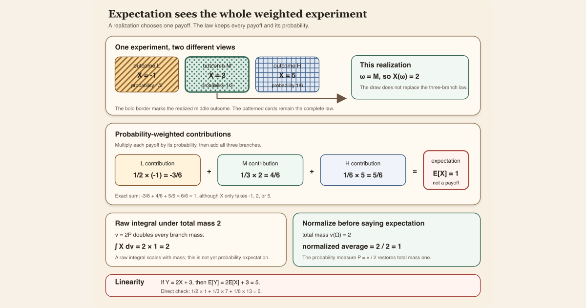
For an integrable real-valued random variable \(X\), its expectation is the integral \(\int X\,d\mathbb P\). A nonnegative random variable also has an extended expectation, which may equal \(+\infty\). On a finite or countable discrete space, the integral is a probability-weighted sum over atoms. For an atomless real law, it is not a sum of “the probability of each exact value”: every singleton has probability zero. Expectation is not the result at one outcome, and it need not belong to the range \(X(\Omega)\).
Expectation is an integral with respect to a probability measure . The probability normalization matters: integrating the same quantity against a general measure of total mass \(2\) doubles the raw integral.
Start with three possible payoffs
Let the outcome space be
\[ \Omega=\{L,M,H\}. \]Define a real-valued payoff \(X\) and probability measure \(\mathbb P\) by
| Outcome \(\omega\) | Payoff \(X(\omega)\) | Probability \(\mathbb P(\{\omega\})\) |
|---|---|---|
| \(L\) | \(-1\) | \(1/2\) |
| \(M\) | \(2\) | \(1/3\) |
| \(H\) | \(5\) | \(1/6\) |
The three probabilities add to one:
\[ \frac12+\frac13+\frac16 =\frac36+\frac26+\frac16 =1. \]Suppose one run produces \(\omega=M\). The realized payoff is then
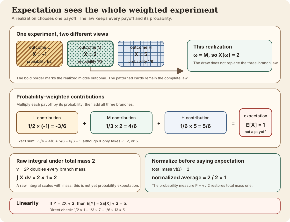
\[ X(M)=2. \]That single observation does not erase the other possibilities. The law of \(X\) still assigns mass \(1/2\) to payoff \(-1\), mass \(1/3\) to payoff \(2\), and mass \(1/6\) to payoff \(5\). A realization is one selected value. In this finite example, the law is the complete weighted list of its three atoms.
Compute the weighted average exactly
On a finite probability space, expectation is the sum
\[ \mathbb E_{\mathbb P}[X] =\sum_{\omega\in\Omega}X(\omega)\mathbb P(\{\omega\}). \]For this payoff,
\[ \begin{aligned} \mathbb E_{\mathbb P}[X] &=\frac12(-1)+\frac13(2)+\frac16(5)\\ &=-\frac36+\frac46+\frac56\\ &=\frac66\\ &=1. \end{aligned} \]The negative payoff contributes \(-3/6\), while the two positive payoffs contribute \(4/6\) and \(5/6\). Expectation combines contributions; it does not choose the most likely payoff.
There is no outcome with payoff \(1\):
\[ X(\Omega)=\{-1,2,5\}, \qquad 1\notin X(\Omega). \]Thus an expectation need not be attainable in a single realization. It is the center of the probability-weighted values, not an additional attained value.
From a finite sum to an integral
For an integrable real random variable
\[ X:\Omega\longrightarrow\mathbb R \]on a probability space \((\Omega,\mathcal F,\mathbb P)\), expectation is
\[ \mathbb E_{\mathbb P}[X] =\int_\Omega X(\omega)\,d\mathbb P(\omega). \]The sigma algebra \(\mathcal F\) specifies the measurable events , and \(\mathbb P\) assigns them probability. The function \(X\) must be measurable so that value-space questions pull back to events. Integrability ensures that the positive and negative contributions combine into a finite real number.
In the three-outcome example, the integral is exactly the weighted sum already computed. The integral notation is not a different average. It is the form that continues to work on continuous and mixed outcome spaces where listing all outcomes is impossible.
Expectation can also be computed from the law \(\mathcal L_{\mathbb P}(X)=X_*\mathbb P\):
\[ \mathbb E_{\mathbb P}[X] =\int_{\mathbb R}x\,d\mathcal L_{\mathbb P}(X)(x). \]The first integral averages over source outcomes. The second averages the identity function over the real value space. They agree because the law is the pushforward of \(\mathbb P\) through \(X\).
Raw mass is not probability expectation
Now define a new measure
\[ \nu=2\mathbb P. \]Its atomic masses are \(1\), \(2/3\), and \(1/3\), and its total mass is
\[ \nu(\Omega)=2. \]The raw integral scales with the measure:
\[ \int_\Omega X\,d\nu =2\int_\Omega X\,d\mathbb P =2. \]This number is not the probability expectation of \(X\) under \(\nu\), because \(\nu\) is not a probability measure. If the intent is to turn a positive finite measure into a probability measure, normalization is an explicit operation:
\[ \widehat\nu=\frac{\nu}{\nu(\Omega)} =\frac{\nu}{2} =\mathbb P. \]The normalized average is then
\[ \frac{1}{\nu(\Omega)}\int_\Omega X\,d\nu =\frac12\cdot2 =1. \]Under a probability measure, the denominator is already one, so expectation is the raw integral. Under a mass-two measure, saying “expectation” without either normalizing or declaring a different convention hides a factor of two.
Linearity: transform first or average first
Expectation is linear. For integrable real random variables \(X\) and \(Z\) and real constants \(a\) and \(b\),
\[ \mathbb E[aX+bZ] =a\,\mathbb E[X]+b\,\mathbb E[Z]. \]A constant function has expectation equal to that constant on a probability space. Therefore, if
\[ Y=2X+3, \]then
\[ \mathbb E[Y]=2\mathbb E[X]+3=2(1)+3=5. \]The direct three-outcome calculation agrees. The transformed payoffs are \(1\), \(7\), and \(13\), so
\[ \frac12(1)+\frac13(7)+\frac16(13) =\frac36+\frac{14}{6}+\frac{13}{6} =\frac{30}{6} =5. \]Linearity does not say \(\mathbb E[XZ]=\mathbb E[X]\mathbb E[Z]\). That product identity requires additional assumptions such as independence and integrability of the product.
In Lean: type the integral that expectation names
∫ ω, X ω ∂μ∫begins Lean’s integral notation.ωis the bound outcome variable. Its scope extends through the integrand that follows the comma.X ωis function application, read as the paper expression \(X(\omega)\).∂μnames the measure used for integration. It is the source notation corresponding to \(d\mu(\omega)\).- The literal line a human places in a Lean file is
∫ ω, X ω ∂μ. The complete worksheet below supplies the import, types, and hypotheses that give every symbol meaning. - The notation itself only forms a raw integral. Calling it an expectation is
semantically justified when
μis a probability measure; a finite real interpretation also requires the appropriate integrability evidence.
The project makes those two gates visible in its finite-horizon cocycle API:
C.finiteHorizonLogPlusExpectation hC kCis a discrete matrix cocycle over the source measureμ.k : ℕis the finite time horizon.C.logPlusNormObservable k ωis the project function \(P_k(\omega)=\log^+\lVert\Phi_k(\omega)\rVert\).hC : C.HasIntegrableGeneratorLogPlusproves the one-step hypothesis from which the project derives integrability at every finite horizon.[IsProbabilityMeasure μ]is present in the complete definition even though it is not printed at the call site. Square brackets ask Lean to synthesize the visible total-mass-one certificate from context.finiteHorizonLogPlusExpectationis a semantic name for the same real integral already calledintegratedLogPlusNorm. It performs no hidden division.
The following definition and theorem are exact excerpts from the checked project source:
def finiteHorizonLogPlusExpectation [IsProbabilityMeasure μ]
    (C : DiscreteMatrixCocycle (ι := ι) μ)
    (_hC : C.HasIntegrableGeneratorLogPlus) (k : ℕ) : ℝ :=
  ∫ ω, C.logPlusNormObservable k ω ∂μ

@[simp] theorem finiteHorizonLogPlusExpectation_eq_integratedLogPlusNorm
    [IsProbabilityMeasure μ]
    {C : DiscreteMatrixCocycle (ι := ι) μ}
    (hC : C.HasIntegrableGeneratorLogPlus) (k : ℕ) :
    C.finiteHorizonLogPlusExpectation hC k = C.integratedLogPlusNorm k := by
  rfl
The underscore in _hC records that the proof is deliberately part
of the interface even though the definition body does not compute with it.
The equality proof is rfl: after unfolding the two project names,
both sides are literally the same integral. The theorem is not a
normalization formula. The probability typeclass has already required total
mass one before the expectation name can be formed.
Try the three-payoff ledger locally
This first worksheet imports only Lean’s small Std library. It
stores every probability as a numerator over the common denominator six, so
the paper calculation
becomes exact integer arithmetic. Save this as
/tmp/ExpectationScratch.lean on a normal Mac or Linux computer:
import Std

namespace ExpectationScratch

def payoffs : List Int := [-1, 2, 5]
def weightsSixths : List Nat := [3, 2, 1]

def contributionsSixths : List Int :=
  List.zipWith
    (fun payoff weight => payoff * Int.ofNat weight)
    payoffs weightsSixths

def totalSixths : Int :=
  contributionsSixths.foldl (fun total term => total + term) 0

def transformedPayoffs : List Int :=
  payoffs.map (fun payoff => 2 * payoff + 3)

def transformedContributionsSixths : List Int :=
  List.zipWith
    (fun payoff weight => payoff * Int.ofNat weight)
    transformedPayoffs weightsSixths

def transformedTotalSixths : Int :=
  transformedContributionsSixths.foldl (fun total term => total + term) 0

#eval contributionsSixths
#eval totalSixths
#eval totalSixths / 6
#eval transformedContributionsSixths
#eval transformedTotalSixths / 6

example : contributionsSixths = [-3, 4, 5] := by decide
example : totalSixths = 6 := by decide
example : totalSixths / 6 = 1 := by decide
example : transformedContributionsSixths = [3, 14, 13] := by decide
example : transformedTotalSixths / 6 = 5 := by decide

end ExpectationScratch
Type these two commands exactly:
source "$HOME/.elan/env"
elan run leanprover/lean4:v4.32.0 lean /tmp/ExpectationScratch.lean
This exact standalone worksheet was executed successfully with Lean 4.32.0. It printed:
[-3, 4, 5]
6
1
[3, 14, 13]
5
The three entries on the first line are the weighted contributions in sixths, not sampled payoffs. The proof lines ask Lean to check the same total and the linearity example \(Y=2X+3\). This bounded worksheet neither imports Mathlib nor constructs a measure-theoretic integral.
Full project check
The next worksheet uses the repository’s Mathlib-backed integral interface. Type it in a clone with the repository’s pinned Lean and Mathlib dependencies installed:
import NonlinearDynamics.Random.RandomCocycles.ProbabilityErgodicBase

open MeasureTheory

#check integral_add
#check NonlinearDynamics.Random.RandomCocycles.DiscreteMatrixCocycle.finiteHorizonLogPlusExpectation
#check NonlinearDynamics.Random.RandomCocycles.DiscreteMatrixCocycle.finiteHorizonLogPlusExpectation_eq_integratedLogPlusNorm

variable {Ω : Type*} [MeasurableSpace Ω]
variable (μ : Measure Ω) (X Y : Ω → ℝ)

#check ∫ ω, X ω ∂μ

example (hX : Integrable X μ) (hY : Integrable Y μ) :
    (∫ ω, X ω + Y ω ∂μ) =
      (∫ ω, X ω ∂μ) + (∫ ω, Y ω ∂μ) := by
  exact integral_add hX hY
The first #check asks for Mathlib’s integral-linearity theorem.
The next two inspect the project’s probability-normalized expectation
definition and its
equality with the raw integrated observable. The local variables make the
line #check ∫ ω, X ω ∂μ meaningful. Finally, the
example supplies explicit integrability proofs to
integral_add, and Lean’s kernel checks the resulting additivity
proof term. It is the typed counterpart of
\(\mathbb E[X+Y]=\mathbb E[X]+\mathbb E[Y]\) when \(\mu\) is a probability
measure, and a valid raw-integral identity for general \(\mu\).
formalization/NonlinearDynamics/Random/RandomCocycles/ProbabilityErgodicBase.lean.
That module imports the finite-horizon log-positive observable and its
integrability theory, requires [IsProbabilityMeasure μ] before
using the expectation name, and proves by rfl that the named
expectation equals integratedLogPlusNorm. The worksheet above uses
the same project import and exact declaration names. The full-project command
checks the complete module with the repository’s pinned dependencies installed.cd formalization
lake env lean -DwarningAsError=true NonlinearDynamics/Random/RandomCocycles/ProbabilityErgodicBase.leanResource note: this exact file uses the repository's
pinned Lean and Mathlib dependencies. Initial project setup can require
substantial disk space and build time. For a lightweight first step on
macOS or Linux, use the page's standalone Lean-core or Std
tutorial.
Distinctions and failure modes
| Tempting shortcut | What is wrong | Correct repair |
|---|---|---|
| “The expectation is what happened” | One realization is \(X(\omega)\); expectation averages the whole law | Keep the observed value and distribution-level average separate |
| “The expectation must be an attained value” | A weighted center can lie between listed atoms and therefore outside the attained finite set | Check the range \(X(\Omega)\) separately |
| “The most likely value is the expectation” | Mode and expectation answer different questions | Compute probability times value for every branch |
| “Any raw integral is an expectation” | A measure may have total mass other than one | Require a probability measure or explicitly normalize a positive finite measure |
| “The law and one sample contain the same information” | One sample selects one value; the law records weights for all values | Use repeated data to estimate the law, not to redefine it after one draw |
| “Finite values guarantee finite expectation” | On an infinite outcome space, tails can make a real random variable nonintegrable | Prove integrability or state an extended nonnegative expectation |
| “Changing a function on a null set changes its expectation” | Integrals identify functions that agree almost everywhere | Use the null set and almost-everywhere interface explicitly |
| “Linearity makes products factor” | \(\mathbb E[XZ]=\mathbb E[X]\mathbb E[Z]\) is not linearity | Add independence and product-integrability hypotheses when appropriate |
Where to continue
Read event for the measurable yes-or-no questions underlying the outcome space. Read measure and probability measure for the difference between raw mass and normalized mass. Read probability law for the value-space distribution that also determines expectation, and null set for changes that do not affect an integral.
The chapter Probability Normalization and Ergodic Rigidity Before Kingman places the project’s finite-horizon expectation beside its integrability and ergodicity assumptions.
References
Mathlib contributors.
Bochner integral basics,
Mathlib 4 documentation. This official implementation reference contains the
real and vector-valued integral API, including integral_add and
the integral of a constant.
Mathlib contributors. Probability measure typeclass, Mathlib 4 documentation. This official source records the total-mass-one assumption used by the project’s expectation interface.
Olav Kallenberg. Foundations of Modern Probability, third edition, Springer, 2021. This is a standard reference for expectation, integration, laws of random elements, and almost-everywhere equivalence.